Returns and Compounding

Main thread: establish what happened in the account before choosing a return measure. Prerequisites are Chapter 2 (Python), Chapter 6 (probability), and Chapter 10 (market instruments). Total return, simple return, log return, means, growth rates, and the Sharpe ratio answer different questions. We start with wealth recursion and proceed to financial-data calculations over matching intervals. All constructed examples are identified; the historical example uses a frozen French monthly release snapshot.

1. Learning objectives

By the end of this chapter, you should be able to calculate simple return and total return from cash and security values, turn returns over consecutive intervals into a wealth path, and explain why log returns add over time but cannot be added directly across assets using capital weights. You should also distinguish the arithmetic mean, geometric mean, and compound annual growth rate (CAGR).

The programming objectives are to retain initial capital, handle a −100% loss and missing values, calculate excess return using the risk-free return for the same month, check drawdown independently, and state the annualization conventions and conditions for volatility and the Sharpe ratio. Finally, read a historical chart and distinguish the descriptions supported by the data from trading conclusions that remain unsupported.

2. Why a quant needs this

A 10% price increase does not always mean a 10% account gain. Dividends, splits, financing, exchange rates, external deposits, and trades within the interval affect the numerator or denominator. A stock falling from 100 to 98 while paying a dividend of 2 does not imply a 2% loss to its holder. Futures notional exposure and margin are also different return denominators. Chapter 10 establishes instrument cash flows; this chapter places them in a common measurement framework.

Signal research needs a specified prediction target: next-month price return, total return, excess return, or log return? Portfolio modules usually use simple returns; statistical models sometimes use log returns; long-term account growth requires compounding. Mixing these objects can make a regression or optimization program optimize the wrong target even when it runs correctly.

We first establish a benchmark account with no external cash flows, one reporting currency, and valuation at each interval end. We then identify the real circumstances that require extending this benchmark. This makes the assumptions visible rather than hiding several of them in one piece of code.

3. Intuition: the percentage denominator changes

An initial 100 rises 50% to 150, then loses 50% of 150 and ends at 75. The two percentages sum to zero, yet the account loses 25%. The second change applies to a different capital base and cannot simply cancel the first.

Currency profit and loss can be added across intervals if both are reported against the same initial 100, but that uses a different denominator convention. A research report must identify the capital base of each return before discussing additivity.

Logarithms turn multiplication into addition, making multi-period growth easier to express. They do not remove risk or merely rename simple return. The change from 100 to 150 gives $\log(1.5)$; from 150 to 75 gives $\log(0.5)$. Their sum is $\log(0.75)<0$, correctly preserving the 25% total loss.

4. Mathematical foundations: accounts, intervals, and units

A monthly label such as 2010-01 normally identifies the January 2010 return interval. It does not establish that a price, signal, or order was known at any particular intraday time. The historical example contains monthly published returns and a current snapshot, with no signals or executions. A strategy backtest must separately specify opening valuation, effective holdings, closing valuation, cash-flow attribution, and data availability and ingestion times.

5. Formal definitions: distinguish the return objects

5.1 Price return and total return

Let $P_{t-1}$ and $P_t$ be the endpoint prices of one unit of a security, and $D_t$ the cash distribution belonging to its holder during the interval. In a simplified example with constant quantity, distributions credited at the interval end, and within-interval reinvestment either negligible or recorded separately,

This requires $P_{t-1}>0$. Prices and distributions use the same currency and per-unit basis. A split that changes quantity must preserve the economic position. If a vendor total-return series already includes dividends, do not add $D_t$ again. Reinvestment, taxes and fees, or multiple distributions within the interval require a complete wealth ledger; this endpoint formula is not a universal formula for corporate actions.

5.2 Arithmetic mean, geometric mean, and CAGR

For $T$ equal-length intervals with simple returns $R_1,\ldots,R_T$, the sample arithmetic mean is

It describes the sample average of a single-interval return, rather than the compounded growth of a path. The geometric mean is

The second expression requires every $R_t>-1$. If one interval has return −1 and no later external capital is injected, terminal wealth is zero and the product definition gives a geometric mean of −1. A finite-log implementation cannot handle this boundary.

For wealth changing from $V_0>0$ to $V_T\geq0$ over $Y>0$ years with no external cash flows, define

$Y$ is an explicit time convention. A regular monthly sample can be reported using a “$T/12$ years under the monthly-interval convention.” Exact calendar time requires dates and a year-length convention. Dividing the row count of irregular data by 252 is not a time definition.

5.3 Excess return, volatility, and the Sharpe ratio

For the same interval and currency, let $R_t$ be the asset simple total return and $R_{f,t}$ the risk-free simple return. Arithmetic excess return is

It compares investing the same capital in the asset and the risk-free account. Growth relative to risk-free wealth is $(1+R_t)/(1+R_{f,t})-1$, which generally differs from $e_t$. Do not substitute relative wealth growth into the ordinary Sharpe numerator.

The sample standard deviation uses $T\geq2$:

The single-interval sample Sharpe ratio is $\widehat{SR}=\bar e/s(e)$. The denominator is the standard deviation of excess returns, rather than an unspecified asset-return standard deviation. When $s(e)=0$, the sample Sharpe ratio is undefined; do not return infinity and call it an ideal strategy. Chapter 32 addresses sampling uncertainty and selection bias.

6. Derivations: from wealth recursion to aggregate risk

6.1 Compounding and log additivity

Substitute $V_t=V_{t-1}(1+R_t)$ repeatedly. For two intervals, $V_2=V_0(1+R_1)(1+R_2)$; induction gives

Total return $R_{0:T}$ uses initial wealth as its denominator. Taking logs of positive wealth and applying the product rule gives

This is an identity. It does not require independent and identically distributed (IID), normal, or stationary returns. It requires one consistent account path, consistent cash-flow attribution, and positive wealth.

6.2 Why the geometric mean does not exceed the arithmetic mean

For positive $1+R_t$, the natural logarithm is strictly concave. Jensen's inequality gives

The exponential function is increasing, so $G\leq\bar R$. Equality holds when all interval returns are equal. This is a sample inequality for the same realized values; it does not establish that every high-volatility asset must grow more slowly than any low-volatility asset, because means and distributions may also differ.

For small $|R|$, the Taylor expansion from Chapter 4 gives $\log(1+R)\approx R-R^2/2$. The sample mean log return is therefore approximately

The squared term contains both sample variance and the squared mean. “Volatility drag” interprets a local approximation; it does not mean subtracting exactly half the variance for every distribution. Large losses, heavy tails, and returns near −100% can invalidate a low-order approximation.

6.3 Cross-sectional portfolios start with simple returns

For two assets with beginning-of-interval capital weights $w_1,w_2$ summing to one, no rebalancing within the interval, and no additional cash flows or financing, terminal wealth is

$w_i$ are beginning-of-interval capital weights, not terminal weights after return-induced drift. Portfolio log return is

It generally differs from $\sum_iw_i\log(1+R_{i,t})$. If two equally weighted assets gain 50% and lose 50% in the same interval, portfolio simple and log returns are both zero, but the weighted asset log returns equal $\frac12\log(0.75)\approx-0.143841$. Aggregation across assets and aggregation across time cannot be interchanged.

6.4 What square-root annualization assumes

More generally, let weakly stationary increments $X_t$ have mean $\mu$, finite variance $\gamma_0$, and lag covariance $\gamma_k$. Expanding the double sum gives

The diagonal contributes $q$ variance terms. Observations $k$ intervals apart form $q-k$ pairs, and the reverse direction contributes the same covariance, producing the factor two. Positive correlation usually increases aggregate variance and negative correlation can reduce it; the full lag structure matters, not just one correlation coefficient.

This formula describes the sum of increments exactly. Log returns add over time, whereas compounded simple return is a product minus one; their standard deviations are not the same exact object. “Monthly return standard deviation times $\sqrt{12}$” may be reported as a conventional annualized measure, with the model and approximation limits stated.

In the same additive model, the $q$-interval mean is $q\mu$, while its risk denominator follows the formula above. The mean-to-standard-deviation ratio reduces to $\sqrt q\,\mu/\sqrt{\gamma_0}$ only when the weighted covariance sum at that horizon is zero. Nonstationary, serially correlated, compounded returns and risk-free returns at different frequencies do not yield an exact annual Sharpe ratio by changing a frequency constant.

7. Financial interpretation: growth, risk, and opportunity cost

The arithmetic mean answers “What is the average single-interval return?” The geometric mean describes growth along an equal-interval path; CAGR compresses initial wealth, terminal wealth, and elapsed time. CAGR does not retain ordering: rearranging the same returns preserves terminal wealth and the geometric mean but can change drawdown and liquidity pressure. An investor's ability to reach the endpoint depends on the path.

The risk-free account is an opportunity-cost benchmark. Compare a monthly asset return with risk-free return for the same month; do not subtract a full-year 4% from every monthly observation. Given a 4% effective annual rate and the additional assumption of constant monthly compounding, the effective monthly rate is $1.04^{1/12}-1$, approximately 0.327374%. Money-market simple-rate quotations, day-count conventions, or actual monthly Treasury-bill returns require their own terms rather than the same exponent formula.

A domestic-currency investment in a foreign asset also involves the exchange rate. Let $S_t$ be the domestic-currency price of one unit of foreign currency and $R_t^{F}$ the foreign-currency asset total return. Ignoring taxes, fees, and hedging,

$H$ denotes domestic currency and $F$ foreign currency; quotation direction determines the exchange-rate factor. A foreign asset gaining 10% while its currency loses 10% against domestic currency gives domestic return $1.1\times0.9-1=-1\%$, not zero. Hedging costs and forward cash flows require a separate ledger.

8. Numerical Example

8.1 Symmetric percentages do not produce symmetric wealth

Construct two years: +50% in year one and −50% in year two. Initial wealth 100 ends at 75. The annual arithmetic mean is 0%, two-year total return is −25%, and the annual geometric mean and CAGR are both −13.3974596%. Year-two drawdown from the historical peak of 150 is −50%; total loss and peak drawdown use different denominators.

8.2 Dividends and external deposits

Construct a price change from 100 to 98 with a dividend of 2 paid at the interval end, no reinvestment, and no taxes or fees. Price return is −2% and total return is 0%. Adding 2 again to a series that already includes dividends would count the cash flow twice.

Another account starts at 100, earns 10% to reach 110, then receives an external deposit of 90 and ends at 200. The 100% increase from 100 to 200 is not investment return. Removing the end-of-interval deposit leaves investment return of 10%. A deposit within the interval cannot be assumed to occur at its end. The challenge exercise below explains segmented time-weighted and money-weighted returns.

8.3 A serial-correlation counterexample for additive increments

Construct weakly stationary increments with monthly standard deviation 0.02 and lag covariance $\gamma_k=0.0004(0.5)^k$. These are theoretical teaching inputs, not actual security returns. The variance multiplier for a 12-interval sum is

Its standard deviation is 0.1131388113, compared with 0.0692820323 from square-root-of-12 scaling that ignores correlation: approximately 63.30% larger. This example checks risk aggregation for a sum of increments; it is not a compounded account or an empirical Sharpe estimate.

8.4 Covariance cancellation at a fixed horizon

8.5 Returns and path risk from an endpoint ledger

9. Python Implementation

Default execution entry point for this reader edition

From the accepted I3 reader package root, create a separate environment using its environment instructions, then run:

.venv/bin/python run_notebook.py notebooks/ch11_returns.ipynb

The Notebook calls the implementation shared within the package. Chapter 11 executes a constructed wealth path by default. French historical loading, plotting, and cache checks remain in skipped explanatory cells rather than default execution. The runner writes fresh-kernel execution records to a unique runs/execution_* directory; new Notebook figures go to a separate UUID directory. The terminal prints the actual locations. French data absent from the package are neither loaded by default nor downloaded. The old course-production tests and historical CLI below refer to the course working root; readers use assertions in the Notebook above. Optional historical data also follow the data contract. This batch did not rerun them.

Historical course working root and original implementation

Core functions are in performance.py; frozen monthly input loading is in market_data.py; the standalone entry point is ch11_returns.py. Cached historical returns are already decimals and are not divided by 100 again. This CLI requires the course root's frozen French files and manifests, rather than serving as the offline default above. The original route is:

.venv/bin/python code/ch11_returns.py

The following constructed example can be run independently from the course root:

import sys
sys.path.insert(0, "src")
import numpy as np
from quant_course.performance import (
    wealth_index, geometric_mean_return, cagr, drawdown_path
)

returns = np.array([0.5, -0.5])
wealth = wealth_index(returns, initial_capital=100.0)
print(wealth)
print(returns.mean(), geometric_mean_return(returns))
print(cagr(100.0, wealth[-1], elapsed_years=2.0))
print(drawdown_path(wealth))
np.testing.assert_allclose(wealth, [100.0, 150.0, 75.0])
np.testing.assert_allclose(drawdown_path(wealth), [0.0, 0.0, -0.5])

# Bridge from chapter2: exclude only the structural initial position.
import pandas as pd
from quant_course import compute_returns
prices = pd.Series([100.0, 110.0, 99.0],
    index=pd.date_range("2026-01-02", periods=3, freq="B", tz="UTC"))
price_returns = compute_returns(prices, kind="simple")
assert pd.isna(price_returns.iloc[0])
interval_returns = price_returns.iloc[1:]
if interval_returns.isna().any():
    raise ValueError("unknown holding interval; do not drop gaps")
price_path = wealth_index(interval_returns.to_numpy(), prices.iloc[0])
np.testing.assert_allclose(price_path, prices.to_numpy())
assert len(price_path) == len(prices) == len(interval_returns) + 1

This bridge applies only to a teaching price path with complete, consistently defined prices and no omitted cash flows. compute_returns retains the initial NaN; wealth_index accepts only simple returns over actual intervals. Exclude only the first entry by position and explicitly check for remaining missing values. Do not use dropna() to delete unknown intervening intervals. Choosing the opening price as initial capital merely reproduces the example's price values; it does not turn price return into total return. Chapter 2 uses r for log return and this chapter uses g for the same natural-log transformation. Neither belongs in wealth_index, which requires simple returns.

Distinguish endpoints from intervals when counting: wealth 100, 150, 75, 120 gives four valuation endpoints but three actual returns, 50%, −50%, and 60%. Initial wealth 100 has no preceding value and is not a market zero return. Retain it in wealth and drawdown paths, but exclude it from return means, volatility, Sharpe samples, and CAGR elapsed time. A displayed initial ret=0 row must be explicitly excluded as a baseline; genuine 0% holding-period returns remain. Missing intervals are unknown observations, which cannot be removed by the initial-row rule.

The wealth output has one more entry than the number of return observations. Its first entry is declared initial capital, not a fabricated market price. A −100% return may reduce wealth to zero; subsequent multiplication cannot restore positive wealth without capital injection. After wealth reaches zero, that account's own subsequent returns have a zero denominator and are undefined. Multiplying hypothetical growth factors afterward only illustrates that zero wealth stays zero, not actual account returns. The added drawdown_path permits zero wealth; the time-indexed compute_drawdown in timeseries.py retains its positive-wealth contract (not developed in Chapter 2). Do not silently interchange them.

All measures reject NaN, infinity, and invalid numeric types rather than applying dropna() automatically. A missing return may represent an unknown wealth change; deleting it joins nonconsecutive intervals. Only a declared, justified research subsample can change the path. “Enough observations remain” is not a substitute for that decision.

RF requires an explicit vector of matching length and intervals; an annual rate is not broadcast automatically. Zero excess-return volatility makes the Sharpe ratio undefined. Extreme values can overflow float64 variance; the function rejects the result rather than misreporting an infinite standard deviation as Sharpe zero. The functions do not identify trading calendars or publication times. The monthly loader verifies hashes, indices, and continuity; the researcher specifies the information clock and execution contract.

10. Visualization

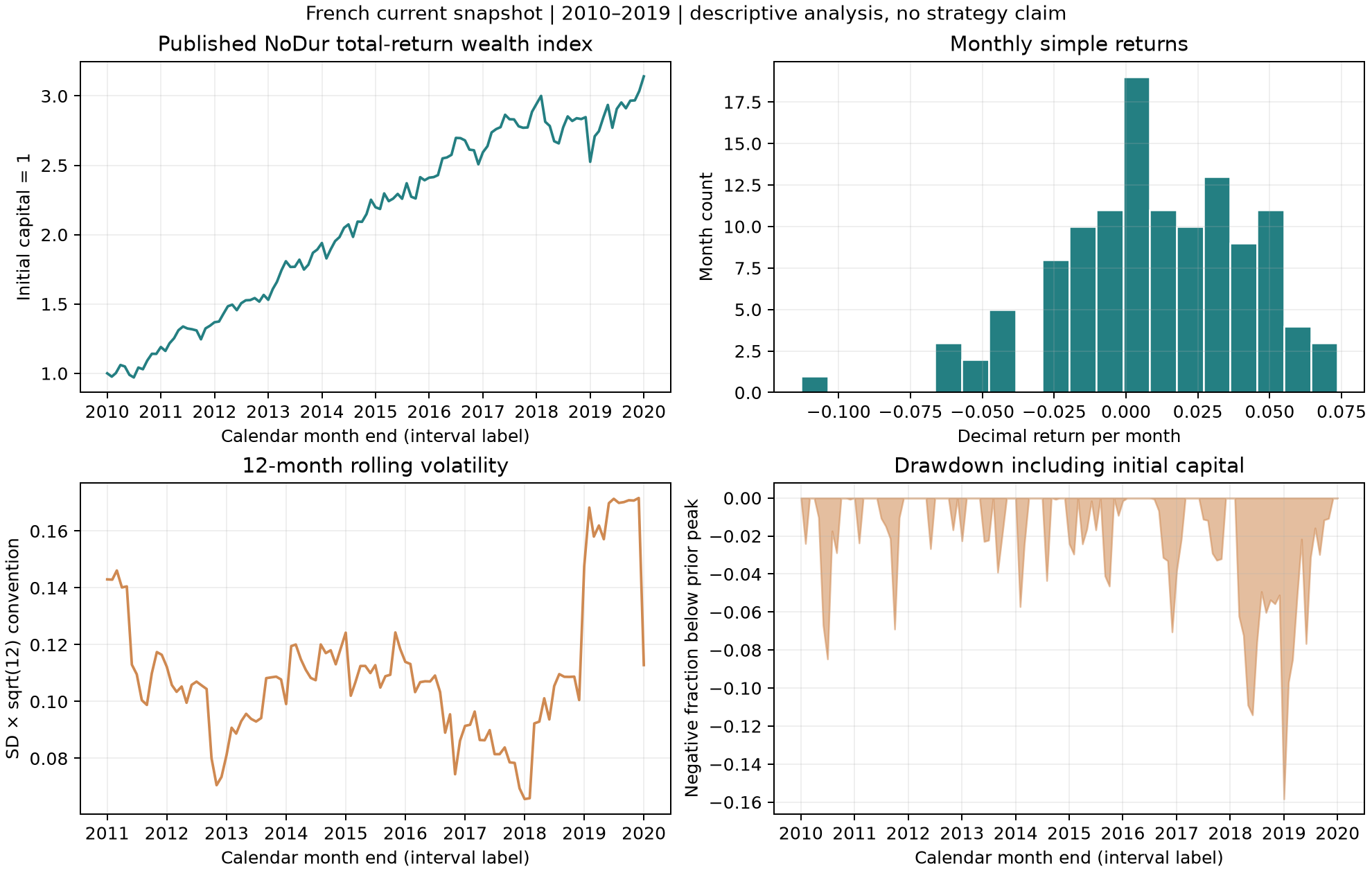
The four panels use the same monthly sample from 2010-01 through 2019-12 and the same calculation code.

• Upper left: the horizontal axis is calendar month-end labels; the vertical axis is a total-return wealth index starting at one. The first point at 2009-12 is chosen initial capital, not an actual 2009 stock price. Examine growth and intervening stagnation rather than judging risk from terminal wealth alone.
• Upper right: the horizontal axis is decimal monthly simple return; the vertical axis counts months in each bin. This is a 120-month frequency histogram, not proof of a population density. Extreme losses and asymmetry require more data and statistical tests.
• Lower left: the horizontal axis is month-end; the vertical axis is the preceding 12 months' sample standard deviation times the square root of 12, a conventional annualized measure. The curve starts only after 12 observations. It uses no future window and does not establish next year's volatility.
• Lower right: the horizontal axis is month-end; the vertical axis is negative drawdown from the highest wealth observed by that month. Zero indicates a new or matched high. The deeper decline in 2018 shows why terminal growth does not eliminate pressure along the path.

The wealth index compounds published portfolio returns. It is not a fund NAV, a stock-level price series, a strategy net of fees, or a product immediately available for purchase.

11. Real Market Example

The sources are Kenneth R. French Data Library's 10 Industry Portfolios and Fama/French 3 Factors. We select published monthly value-weighted industry portfolio returns in the NoDur column. RF is the same-month FF3 Treasury-bill return proxy; it is not assumed to equal a frictionless cash rate available to every investor. NoDur identifies the nondurable-consumer-goods industry portfolio, not a security ticker.

The processed caches' month labels and hashes are verified against their respective manifests. A one-to-one monthly join over 2010-01 through 2019-12 gives 120 months, with no imputation or frequency mixing. Initial capital is one. The script calculated the following values; return units are decimals:

These values describe this specified interval in the current published version. The 2010–2019 window is for teaching, not an independently validated preferred investment period. It defines no exit rule, signal, order, or cost model. Portfolio constituent treatment, return methodology, and historical revisions belong to the publisher; they do not establish a stock-level historical universe built by this project.

The manifests record download times and hashes from 2026-10-05. Historical data downloaded in 2026 do not establish that researchers in 2010 saw the same version. Complete point-in-time publication and ingestion histories have not been built. This is retrospective descriptive analysis and makes no claim that look-ahead bias has been eliminated at the trading level.

12. Common Mistakes

Adding returns and calling the sum total return. The incorrect calculation +50%−50%=0 ignores the changing denominator. Correct total return is $(1.5)(0.5)-1=-25\%$. Adding currency profit and loss requires a consistent capital basis and stated account cash flows.

Adding dividends again to total return. Adjusted prices do not necessarily use the same total-return convention. Read the vendor definition and Chapter 3's corporate-action contract first. Distributions already included cannot be credited twice. Split adjustment preserves the relation between quantity and price; it creates no economic return.

Deleting blank months before compounding. Missing is neither zero nor a market pause. If the account's wealth change is unknown, terminal wealth and maximum drawdown are not fully determined. Current core functions raise an error rather than silently joining nonadjacent intervals.

Calling annualized output a forecast of next year's risk. Square-root-of-time scaling depends on risk aggregation conditions; a rolling sample describes its historical window. Forecasting next year requires a model, estimation uncertainty, and out-of-sample evaluation. Chapter 18 develops dynamic volatility models.

Treating net deposits as investment profit. CAGR applies only to the declared path without external cash flows. With inflows and outflows, segmented time-weighted and money-weighted returns answer different questions. Recording cash-flow times matters more than choosing an attractive percentage.

13. Quant Research Application

First define the target object, frequency, and interval. For next-month total return, distinguish feature time from label end time: a training label is complete only once its interval has ended and it is available. When converting a log-return prediction to simple return, consider the distribution and estimand. $\exp(E[g])-1$ generally differs from $E[\exp(g)-1]$; exponentiating a predicted mean does not automatically give expected simple return.

Next determine the account denominator. A portfolio backtest applies effective beginning-of-interval capital weights to subsequent asset total returns, then subtracts fees and financing to form net wealth. Self-financing constraints, cash holdings, stock borrowing, and derivative notional exposures require a ledger. Convert annual RF and foreign-currency benchmarks to matching intervals and definitions before subtraction; matching column names is insufficient.

Report mean, growth, volatility, drawdown, sample scope, and costs together. Store calculation values as decimals and convert to percentages for display. Retain raw and processed versions, hashes, missing-data rules, and measurement intervals. Project 1 uses these steps for a descriptive financial-data report; Chapter 29 develops execution and holdings ledgers.

14. Chapter Summary

Simple return connects neighboring wealth values. Log return turns temporal multiplication into addition on a positive-wealth path; cross-asset portfolios still start with simple returns and beginning-of-interval capital weights. The arithmetic mean describes single-interval sample returns; the geometric mean and CAGR summarize compound growth; drawdown preserves peak-to-trough path information.

Annualization involves more than changing a display unit. The variance of summed increments depends on all lag covariances. Square-root time is either scaling under specific conditions or an explicitly stated convention. RF, distributions, external deposits, currency, and the measurement clock determine what an indicator means. Define them before interpreting figures and values.

15. Exercises

11-E01 (Concepts) Explain the differences between simple return, log return, price return, and total return. State the account or cash-flow conditions for each.

11-E02 (Hand calculation) Start at 100, gain 50%, then lose 50%, with each interval lasting one year. Calculate terminal wealth, total return, arithmetic mean, geometric mean, CAGR, and maximum drawdown.

11-E03 (Portfolio) Two equally weighted assets gain 50% and lose 50% in one interval. Calculate portfolio simple and log returns, weighted asset log returns, and terminal capital weights. Explain the difference between time and cross-sectional aggregation.

11-E04 (RF) Monthly asset return is 2% and monthly RF is 0.3%. Calculate arithmetic excess return and growth relative to risk-free wealth. What monthly effective rate corresponds to an effective annual rate of 4% under constant monthly compounding?

11-E05 (Currency) A foreign-currency asset gains 10%, while the domestic-currency price of one foreign-currency unit falls 10%. Calculate domestic total return and explain why quotation direction matters.

11-E06 (Annualization) Derive the variance of a $q$-interval increment sum from the covariance double sum. What conditions does square-root-of-time scaling require? Why is it not the exact risk formula for compounded simple return?

11-E07 (Path) Compare three-interval returns $(50\%,-40\%,-20\%)$ and $(-40\%,50\%,-20\%)$, starting at 100. Are terminal wealth, CAGR, and maximum drawdown the same?

16. Programming Exercises

11-P01 (Wealth boundaries) Use the core functions to check +50%/−50%, a one-interval −100% loss, and NaN input. What is the initial point? Why cannot a positive percentage restore wealth after bankruptcy?

11-P02 (Risk aggregation) For $\gamma_k=0.0004(0.5)^k$ in Section 8.3, calculate the standard deviation of a 12-interval sum and the scaling that ignores serial correlation. Do not call the result an actual strategy's annual Sharpe ratio.

11-P03 (Historical cache) Run the frozen-cache analysis; verify the same-month NoDur/RF join, 120 consecutive months, terminal wealth, and indicators. Produce at least one chart and write three supported interpretations and two limitations.

17. Challenge Problems

11-C01 (Approximation and inequality) Prove that the equal-interval geometric mean does not exceed the arithmetic mean. Explain equality, the conditions for $\bar g\approx\bar R-\overline{R^2}/2$, and why “geometric mean equals mean minus half the variance” is not exact. Ten points: concavity and Jensen (4), exponential monotonicity and equality (2), Taylor range and second-moment term (2), extreme-return boundaries (2).

11-C02 (External cash flows) Split a year into two halves. Initial 100 earns 10% to 110; a deposit of 90 brings capital to 200; the second half earns 10% to 220. Calculate time-weighted return (TWR) and compare it with the unadjusted terminal-to-initial ratio. Write the cash-flow equation for money-weighted return and explain the difference. Ten points: segmented capital (2), TWR product (3), incorrect ratio (1), internal rate of return (IRR) equation and timing (2), the questions answered by the two returns (2).

11-N01 (Variance scaling at a fixed horizon) For weakly stationary, equal-variance increments, derive the necessary and sufficient condition for exact square-root scaling at a specified horizon $q$ from the covariance double sum. Explain what the condition implies if it holds at every horizon. Use the Section 8.4 matrix to verify three-interval cancellation and matrix validity, then compare the two-interval result. State why this establishes neither independence nor a universal variance formula for compounded simple returns.

18. Solutions / Solution Hints

11-E01 Answer. Simple return divides the change between neighboring wealth values by beginning wealth; the benchmark account has no external inflows and positive initial wealth. Log return is the natural log of a positive wealth ratio and adds over time, requiring positive terminal wealth as well. Price return tracks only prices; total return includes attributed distributions and other investment cash flows. Splits must preserve the economic position, and within-interval reinvestment requires a ledger. Do not add dividends to a series that already includes distributions. Log return is not synonymous with total return: one may take logs of either total-return wealth or a price path, but their cash-flow coverage remains different.

11-E02 Answer. Wealth is 100, 150, 75. Total return is −25%, arithmetic mean is 0%, and the geometric mean and CAGR are $\sqrt{0.75}-1=-13.3974596\%$. Drawdown from peak 150 to terminal 75 is −50%; maximum drawdown may be reported as a positive loss magnitude of 50%. It differs from the 25% loss against initial capital.

11-E03 Answer. Initial weights are 0.5 each. Portfolio simple return is 0.5×0.5+0.5×(−0.5)=0, so portfolio log return is $\log1=0$. Weighted asset log return is $\frac12[\log1.5+\log0.5]=\frac12\log0.75\approx-0.143841036$, not zero. Terminal capital is 75 and 25, with weights 0.75 and 0.25. Those weights describe the next interval's starting allocation, not this interval's return.

11-E04 Answer. Arithmetic excess return is $0.02-0.003=0.017$, or 1.7%. Growth relative to risk-free wealth is $1.02/1.003-1\approx0.0169491525$, approximately 1.694915%. The monthly effective rate is $1.04^{1/12}-1\approx0.0032737398$, or 0.327374%. This conversion assumes constant compounding and cannot be inferred from an arbitrary annualized quotation.

11-E05 Answer. The domestic growth factor is 1.1×0.9=0.99, giving total return −1%. A lower domestic-currency price of one foreign-currency unit means foreign-currency depreciation. If the quotation instead gives foreign currency per domestic unit, invert the conversion factor rather than continuing to multiply by 0.9. The example ignores hedging, taxes, fees, and trading costs.

11-E06 Answer. The diagonal has $q$ terms of $\gamma_0$ each. Positive lag $k$ has $q-k$ pairs, with equal symmetric contributions at negative lags, giving $q\gamma_0+2\sum_{k=1}^{q-1}(q-k)\gamma_k$. With equal interval variances, exact square-root scaling at specified $q$ holds if and only if $\sum_{k=1}^{q-1}(q-k)\gamma_k=0$. Zero cross-interval covariances suffice but are not necessary at a fixed horizon because positive and negative terms can cancel. If scaling must hold at every horizon, weak stationarity requires every nonzero-lag covariance to vanish. Independence suffices but is not necessary. Compounded simple return is $\prod(1+R_t)-1$, not an increment sum, so this is not its general exact variance formula. Log returns can be added, but then the risk object has changed.

11-E07 Answer. The first path is 100→150→90→72, with maximum drawdown $1-72/150=52\%$. The second is 100→60→90→72, with maximum drawdown $1-60/100=40\%$. Both end at 72, giving total return −28%. If each interval is one year, both CAGRs are $0.72^{1/3}-1\approx-10.37\%$. Ordering does not change the product, but it changes intervening peaks and troughs; equal endpoints do not imply equal holding experiences or risks.

11-P01 Reference implementation.

import sys
sys.path.insert(0, "src")
import numpy as np
from quant_course.performance import wealth_index, drawdown_path

first = wealth_index([0.5, -0.5], 100.0)
bankrupt = wealth_index([0.1, -1.0, 10.0], 100.0)
np.testing.assert_allclose(first, [100, 150, 75])
np.testing.assert_allclose(bankrupt, [100, 110, 0, 0])
np.testing.assert_allclose(drawdown_path(bankrupt), [0, 0, -1, -1])
try:
    wealth_index([0.1, np.nan], 100.0)
except ValueError:
    print("missing interval rejected")
else:
    raise AssertionError("unknown return cannot be silently removed")

The first point is explicitly chosen capital before the interval. Zero times any finite growth factor remains zero. External capital injection is a separate cash flow to record, not a larger next-interval return.

11-P02 Reference implementation.

import numpy as np
q = 12
variance_per_month = 0.0004
rho = 0.5
lags = np.arange(1, q)
variance_sum = variance_per_month * (
    q + 2 * np.sum((q - lags) * rho**lags)
)
actual_sd = np.sqrt(variance_sum)
zero_cov_sd = np.sqrt(q * variance_per_month)
print(actual_sd, zero_cov_sd)
assert np.isclose(actual_sd, 0.11313881131159192)
assert np.isclose(zero_cov_sd, 0.06928203230275509)

The declared theoretical increment sum has standard deviation 0.1131388113, versus 0.0692820323 with zero covariance. The difference comes from lag covariances. No security data, account implementation, or trading rules are involved.

11-P03 Reference implementation.

import runpy
import numpy as np
lesson = runpy.run_path("code/ch11_returns.py", run_name="lesson_functions")
sample = lesson["monthly_example"]()
result = lesson["summarize_monthly"](sample)
assert len(sample) == 120
assert sample.index[0].strftime("%Y%m") == "201001"
assert sample.index[-1].strftime("%Y%m") == "201912"
assert not sample.isna().any().any()
np.testing.assert_allclose(result["wealth_final"], 3.141190294871468)
lesson["make_figure"](sample, lesson["ROOT"] / "figures/a3/ch11_returns_dashboard.png")
print(result)

This example reuses the standalone entry point's input/output and plotting wrappers; the numerical core calls performance and market_data in src. Interpretations may state that selected-window wealth rises from one to about 3.141, month-end drawdown deepens around 2018, and rolling volatility changes with the sample window. Limitations include month-end sampling missing intraday or between-day maximum drawdown, the current release not reconstructing contemporaneous data versions, no executable holdings or costs, and a teaching window not establishing superior investment selection. Grade open responses on correspondence to chart or values and specific conditions and evidence limits.

11-C01 Reference argument. For $R_t>-1$, $\log$ is strictly concave. Jensen gives $\overline{\log(1+R)}\leq\log(1+\bar R)$; exponential monotonicity implies $G\leq\bar R$. Equality requires identical realized returns. The local second-order Taylor expansion is $\bar g\approx\bar R-\overline{R^2}/2$, while $\overline{R^2}=\overline{(R-\bar R)^2}+\bar R^2$. One cannot subtract only sample variance or equate $\bar g$ directly with $G$: exponential conversion and higher-order error remain. Near −1, logs and higher-order terms change sharply; exactly −1 has no finite logarithm. The arithmetic–geometric mean inequality for nonnegative growth factors can cover the zero-growth boundary, but the finite-log proof requires a separate limiting argument.

11-C02 Reference argument. The first-half growth factor is 1.1. The deposit changes capital to 200, and second-half growth is 220/200=1.1. TWR is 1.1×1.1−1=21%. The unadjusted 220/100−1=120% mixes the external 90 with investment profit.

From the investor's perspective, cash outflows are 100 at time zero and 90 at 0.5 years, with an inflow of 220 at one year. The IRR equation for annual effective money-weighted return $r$ is

Set $z=\sqrt{1+r}>0$ and multiply by $z^2$ to obtain $100z^2+90z-220=0$. The positive root is $z=(-90+\sqrt{96100})/200=1.1$, so $r=21\%$. Both halves earn 10%, making the effective annual return unaffected by deposit timing in this example, so the two measures coincide. They still answer different questions: TWR excludes the scale of external flows, whereas IRR reflects investor cash-flow amounts and timing. If second-half return changes to −10%, terminal wealth is 180 and TWR=−1%. Replacing terminal cash with 180 in the IRR equation gives $r\approx-6.8587\%$ from the positive root; the measures differ. Specifically, $z=(-90+\sqrt{80100})/200$, then $r=z^2-1$.

11-N01 Reference argument. Under weak stationarity with interval variance $\gamma_0$, the covariance double sum is $q\gamma_0+2\sum_{k=1}^{q-1}(q-k)\gamma_k$. At fixed $q$, it equals $q\gamma_0$ if and only if $\sum_{k=1}^{q-1}(q-k)\gamma_k=0$. If the condition holds at every horizon, $q=2$ first implies $\gamma_1=0$, and recursion over horizons implies zero covariance at every nonzero lag. The Section 8.4 leading principal minors are $1$, $0.99$, and $0.936$, all positive, so the matrix is positive definite. At $q=3$ the weighted sum is $2(0.1)-0.2=0$ and three-interval variance is three; at $q=2$ variance is $2+2(0.1)=2.2$. The positive and negative covariances cancel only over these three intervals. This establishes neither independence nor square-root scaling at other horizons. The formula concerns a sum of increments, not a universal variance formula for compounded simple returns.

19. Further Reading

• Must Know: MIT OCW 15.401 compounding lecture, effective annual rates on slides 28–29 and real/nominal cash-flow consistency on slides 30–34.
• Should Know: French industry portfolio methodology and FF3 factor/RF descriptions. Use cache manifests to distinguish total returns, factor spreads, and RF.
• Advanced: Andrew W. Lo (2002), The Statistics of Sharpe Ratios, author publication record and abstract. Only metadata and the abstract were checked; the full text was not obtained. Consult the original equations when Chapter 32 develops Sharpe inference.
• Optional: Chapter 3 (corporate actions and dual clocks), Chapter 18 (dynamic volatility), Chapter 29 (ledgers), and Chapter 32 (statistical evaluation) progressively extend the no-external-cash-flow benchmark.

20. References

The actual external-source reading scope is recorded in source_notes.md and the source/metric preparation contract. The compounding source is MIT's official course. The risk aggregation formula is independently derived here by covariance expansion, not attributed equation by equation to an unread Lo full text.

Data versions, download times, units, and SHA-256 values are recorded in the industry manifest and FF3/FF5 manifest. Checkable values are in the actual metric output. Wealth and charts are original calculations, not copied source figures. Public download availability was not treated as permission to redistribute all data.