Transaction Costs

Prior engineering evidence is cited under its original acceptance status. Through-line: map optimizer target weights and ideal prices through spread, slippage, impact, fees, financing, and borrow costs to scenario-specific fill quantities, cash changes, and ending net asset value (NAV). Prevent frictions already embedded in fill prices from being charged again as cash expenses, and establish self-financing and capacity-sensitive boundaries for net-return accounting. Prerequisites: Chapter 29, Backtest Ledgers; and Chapter 34, Market Microstructure. After reading, you should be able to separate the pricing logic for commissions, spreads, slippage, temporary impact, and permanent impact; derive the closed-form purchasable quantity under a self-financing constraint; post cash entries without double counting; hand-reconcile a complete implementation-shortfall ledger with partial fills and multi-asset frictions; and build turnover and capacity sensitivity analyses, including a strategy's break-even AUM.

1. Learning Objectives

In quantitative investing and multifactor research, paper portfolios and portfolios net of costs use different assumptions about fills and expenses. An optimizer that ignores execution constraints may recommend turnover beyond what a strategy can support. Realized results also depend on spreads, impact, commissions, financing, borrow, execution windows, and fill data. The examples in this course use explicit constructed inputs to demonstrate accounting methods; they do not describe a real strategy or market sample.

After completing this chapter, you should be able to demonstrate five professional competencies:

1. Cost categories and units. Distinguish explicit fees (commissions, exchange fees, and taxes), implicit costs (bid-ask spread, slippage, temporary impact, and permanent impact), and position-carry costs (financing interest and borrow fees). Use USD per share, shares, total cash in USD, basis points (bps, where $1\text{ bps}=0.01\%=10^{-4}$), and annualized percentages consistently; do not mix dimensions in an equation.
2. Avoiding double charges and reconciling the ledger. Understand how implicit costs enter the execution price. Prove that once the fill price includes the half-spread and temporary impact, debiting the actual fill notional from cash must not be followed by a second cash debit for spread or impact. Prove that permanent impact changes the subsequent reference-price path and is reflected through valuation, rather than posted again as a cash flow.
3. Solving for self-financing trades. Understand how trading frictions feed back into purchasable asset quantities. Given cash and target weights, write the nonlinear self-financing equation with slippage and fees, and derive the corrected purchase quantity for single- and multi-asset cases so a backtest does not overdraw cash.
4. Reconciling implementation shortfall (IS). Attribute the difference between a paper decision and the executed outcome to delay cost, execution friction, opportunity cost on unfilled shares, and explicit fees. Prove the algebraic decomposition and its equality to the direct cash-difference method.
5. Capacity and calibration boundaries. Apply square-root and linear impact models within their limits; distinguish constructed scenario inputs from empirical calibration to institutional data; and derive the relationship among turnover, AUM, and net returns, including the AUM at which a strategy reaches break-even.

Completion criterion: you can independently hand-calculate the multi-asset example in Section 8 and match its fill quantities, prices, cash balance, fee details, and ending NAV to the cent. You can also identify the code and accounting defects in the double-charge example in Section 12 and state the correct repair.

2. Why Quant Needs It

A quantitative strategy's life cycle runs from a signal to net profit:

[Factor signals / Alpha model]
        |
        v (decision time: signal_time)
[Portfolio optimizer: target weights w*]
        |
        v (order submission and routing: order_send_time)
[Execution algorithm and matching: trade_time] ---> spread, impact, slippage, commission
        |
        v (actual fills: F = Q - R)
[Account and ledger update: fill_time] ---> cash debit/credit, position update, financing/borrow accrual
        |
        v (valuation: mark_time)
[NAV and capacity assessment] ---> determines the capital scale the strategy can support

Ignoring trading costs overstates the net return a paper portfolio can realize:

• High-turnover scenario: Costs accumulate on actual traded notional in the tradable risky assets. Suppose a constructed example invests the entire portfolio in tradable stocks, has one-sided annual turnover $\tau_{\text{turnover}}=15$, and incurs an average cost of 15 bps per dollar of actual traded notional. Using total stock turnover of $2\tau_{\text{turnover}}A$, the cost is about $2\times15\times15=450$ bps of beginning-of-period NAV. Changes in the cash weight do not enter stock traded notional. This is arithmetic only, not a universal input for any strategy or market.
• Liquidity differences: The same share quantity can incur different costs under different quoted depth, volume, and volatility conditions. Without historical order-book and trade data for each security, a researcher can run transparent scenarios but cannot present an assumed spread as a market fact.
• Borrow constraints: Short orders also depend on borrow availability, rates, recalls, and the conditions for buying to cover. Without timestamped historical borrow records, a backtest must use explicit scenario inputs; it cannot assume that every stock is always borrowable.
• Scale sensitivity: As assets under management rise, target orders may become larger relative to available liquidity. How costs scale depends on the execution model and calibration data. This chapter uses constructed functions to illustrate that dependence; it gives no universal capacity threshold.

Chapter 29 established a discrete self-financing ledger, and Chapter 34 unpacked limit order books and market matching. This chapter connects the two: it models spreads and impact, feeds them into Chapter 29's cash ledger, and shows how trading frictions affect portfolio compounding. It also supplies the cost-accounting foundations for Chapter 36's execution methods—TWAP, forecast-volume VWAP, POV, and implementation shortfall.

3. Intuition

3.1 A Used-Car Analogy

A used-car purchase is an intuitive way to think about trading costs. Suppose the fair midpoint valuation of a model is USD 20,000:

1. Bid-ask spread: A dealer will pay USD 19,500 if you sell the car (the bid) and ask USD 20,500 if you buy the same model (the ask). The USD 1,000 difference is the quoted spread. At the USD 20,000 midpoint valuation, a buyer immediately incurs half the spread, or USD 500.
2. Explicit commission and fees: The motor-vehicle authority charges a USD 200 transfer fee and transaction tax. This is an explicit cash expense.
3. Market impact: Suppose you need 50 cars that afternoon to start a rental business, but local dealers have too little inventory and must source more cars at higher prices. The first car costs USD 20,500, the twentieth costs USD 21,000, and the fiftieth costs USD 22,000. Your large, urgent purchase has moved prices against you: this is market impact.
4. Temporary versus permanent impact: After you leave with the 50 cars, the buying pressure subsides and the dealer's ask falls from USD 22,000 to USD 20,800. To compare like with like, suppose the pre-trade midpoint is USD 20,000 and the half-spread is USD 500, so the pre-trade ask is USD 20,500. During the busiest part of the purchase, the ask reaches USD 22,000. If the post-trade ask is USD 20,800 and the half-spread remains USD 500, the corresponding midpoint is USD 20,300. This constructed path labels the USD 1,200 difference between the busy-period ask and the post-trade ask as temporary, and the USD 300 difference between the post-trade and pre-trade midpoints as permanent. It is a specified hypothetical path: a finite observation window cannot establish that impact is permanent or that prices will recover at any particular speed.
5. Financing and stock borrow: If you borrow money from a bank to buy the car, you pay financing interest. If you borrow a friend's car, sell it, and promise to buy another one to return in a month, you pay a rental fee analogous to stock-borrow cost.

3.2 Why You Must Not Charge the Same Cost Twice

A common accounting error is to charge a friction twice. Suppose you buy a car from a dealer for USD 20,500. The fair midpoint value is USD 20,000, so the purchase price already includes the USD 500 half-spread. You also pay a USD 200 transfer fee.

Your cash falls by USD 20,500 + USD 200 = USD 20,700. You receive one car, valued at USD 20,000 at the midpoint. Your net assets therefore fall by USD 700: the USD 500 half-spread plus the USD 200 transfer fee.

The USD 500 spread loss is already reflected in the USD 20,500 purchase price. If backtest code debits USD 20,500 for the car and then separately debits a USD 500 “spread fee,” cash falls by USD 21,200. The spread has been charged twice.

The accounting rule is simple: the fill price absorbs spread and impact, explicit fees are debited separately, and modeled permanent price changes enter through valuation; never post the same cost twice.

4. Mathematical Foundations

Before defining each trading cost, we fix the notation, variable dimensions, and units.

4.1 Core Variables and Dimensions

At a rebalance time, let the portfolio contain $N$ risky assets and one risk-free cash account.

• $P_t^{\text{mid}}\in\mathbb{R}_{++}^N$: midpoint-price vector at time $t$, in USD per share.
• $a_t,b_t\in\mathbb{R}_{++}^N$: best ask and bid vectors, in USD per share, with $b_t<P_t^{\text{mid}}<a_t$.
• $S_t=a_t-b_t\in\mathbb{R}_{++}^N$: quoted spread in USD per share. The relative spread is $s_t=S_t/P_t^{\text{mid}}$, dimensionless or reported in bps.
• $Q\in\mathbb{R}^N$: signed parent-order quantity in shares. $Q_i>0$ is a buy and $Q_i<0$ is a sell.
• $F\in\mathbb{R}^N$: signed filled quantity in shares. It satisfies $|F_i|\le|Q_i|$; when $F_i\ne0$, $\operatorname{sgn}(F_i)=\operatorname{sgn}(Q_i)$. Zero fills are allowed.
• $R=Q-F\in\mathbb{R}^N$: signed cutoff remainder in shares.
• $C_t\in\mathbb{R}$: available cash in USD at time $t$. $C_t<0$ means cash borrowing or leverage.
• $H_t\in\mathbb{R}^N$: holdings in shares at time $t$. $H_{i,t}<0$ means a short position.
• $\text{NAV}_t\in\mathbb{R}$: net asset value in USD, marked at the stated valuation prices.

4.2 Basis Points and Percentages

Small trading proportions are often stated in basis points (bps):

For example, 15 bps equals 0.15% or 0.0015. At a share price of USD 50.00, a 20-bps spread corresponds to an absolute amount of

4.3 From Confirmed Fills to Valuation: Post First, Then Compare Benchmarks

Continue the small connection example from Chapter 34. A request for $Q=100$ shares does not change holdings. Only the actual fill of $F=60$ shares changes cash from USD 2,000 to USD 1,396.70 and shares from 0 to 60. The fill price of USD 10.05 already includes the execution deviation from the quote; debit only the explicit USD 0.30 fee separately. When the mark moves from USD 10.02 to USD 10.10, cash stays unchanged, the position value rises by $60(10.10-10.02)=\text{USD }4.80$, and NAV moves from USD 1,997.90 to USD 2,002.70.

The four IS components for this buy are

The USD 3.20 opportunity cost did not buy any shares, and the USD 2.00 delay cost was not paid to anyone. Both are attribution components. If total IS were debited from cash after the fill had already been posted, NAV would be incorrectly reduced to USD 1,995.40, a second charge of USD 7.30. Section 6.2 proves the general signed identity; Section 8 preserves the full multi-asset, corporate-action, and financing ledger example.

5. Formal Definitions

This section gives the mathematical and financial definitions of the main components of trading costs.

5.1 Commissions and Explicit Fees

Definition 5.1 (Explicit Fees). Explicit fees are cash expenses charged directly for trading activity by a broker, clearing house, exchange, or regulator. Denote them by $\Xi\ge0$, in USD. They commonly include:

1. Per-share commission: $\Xi_{\text{share}}=c_{\text{share}}\sum_i|F_i|$, where $c_{\text{share}}$ is a fee per share (for example, $\$0.005/\text{share}$).
2. Notional commission: $\Xi_{\text{notional}}=c_{\text{notional}}\sum_i|F_i|P_i^{\text{fill}}$, where $c_{\text{notional}}$ is a dimensionless rate (for example, 1.5 bps = 0.00015).
3. Other transaction fees and taxes: where a model includes these items, their schedules must be specified for the relevant venue, product, and account. This chapter makes no claim about the current fee or tax rules of any jurisdiction. The sell-side term in the equation below is an optional modeling term, not a universal legal rule.

The combined explicit-fee function is

Conditions and properties: In this chapter’s ledger model, commission is fill-based and applies only to actual fills $F_i$; an unfilled remainder $R_i$ does not incur the modeled fill commission. Account-specific order-submission or cancellation fees are outside this model.

5.2 Bid-Ask Spread

Definition 5.2 (Effective and Realized Spread). Let an order reach the market at time $t_{\text{arr}}$, when the best bid is $b$, the best ask is $a$, and the midpoint is $P^{\text{mid}}=(a+b)/2$.

1. Quoted spread: $S^{\text{quote}}=a-b$. The relative quoted spread is $s^{\text{quote}}=(a-b)/P^{\text{mid}}$.

2. Effective half-spread cost: For a child order filled at $P^{\text{fill}}$ at time $t$, the one-sided move from the arrival midpoint equals half the spread in the no-impact limit. For signed fill quantity $F$, a buy ($F>0$) executes at the ask and a sell ($F<0$) at the bid:

   $$P^{\text{fill}}=P^{\text{mid}}+\operatorname{sgn}(F)\cdot\frac{S^{\text{quote}}}{2}.$$

   The total spread amount paid on the fill, in USD, is

   $$\text{Cost}_{\text{spread}}=|F|\cdot\frac{S^{\text{quote}}}{2}=F\cdot(P^{\text{fill}}-P^{\text{mid}}).$$

Condition: This formula assumes the order size does not exceed displayed quantity at the best level. When an order consumes multiple levels, depth slippage and market impact must also be considered.

5.3 Slippage

Definition 5.3 (Slippage). Slippage is the adverse deviation of the actual fill price $P^{\text{fill}}$ from a specified reference price $P^{\text{ref}}$:

• If the reference price is the decision-time midpoint $P^{\text{decision}}$, slippage includes market drift during decision delay and all execution frictions after arrival.
• If the reference price is the arrival midpoint $P^{\text{arrival}}$, slippage includes half-spread and immediate market impact.
• The total slippage amount is $F\cdot(P^{\text{fill}}-P^{\text{ref}})$. Positive slippage means execution was worse than the reference benchmark.

5.4 Market Impact: Temporary versus Permanent

A large order can disturb supply and demand and move prices against the trader. Almgren and Chriss (2000) formalized a decomposition of this effect into temporary and permanent impact.

Definition 5.4 (Temporary Impact). A trader demanding immediate liquidity temporarily consumes order-book depth, making the fill VWAP worse than the contemporaneous midpoint in the absence of the trader's order. In this model, this component enters the fill price but not the post-trade reference midpoint. That modeling convention does not establish that real prices recover quickly; recovery speed must be tested with event data.

Suppose a trade is executed at rate $v=|F|/\Delta t$ over a window $\Delta t$. Temporary impact raises a buy price and lowers a sell price:

where $g(|F|,\Delta t)\ge0$ is the temporary-impact function. A common classical specification is a power law:

Fix the volatility measurement window in advance. For example, let $\sigma_{r,1\mathrm d}$ be the sample standard deviation of daily returns over the 60 complete trading days before the decision, excluding post-decision data. Define $\sigma_{P,1\mathrm d}=P_t^{\text{mid}}\sigma_{r,1\mathrm d}$ in USD per share; this is the standard deviation of the one-day price increment. Then $g$ is in USD per share. The coefficient $\eta$ and participation-rate exponent are dimensionless; $V_{\text{slot}}$ is total market volume in the slot; $\eta>0$ is a liquidity coefficient; and $\alpha\in[0.5,1.0]$ is the impact exponent ($\alpha=1$ is linear impact and $\alpha=0.5$ is square-root impact).

Definition 5.5 (Permanent Impact). In this model, a price change attributed to the trader's order and retained in the post-trade reference midpoint is called permanent impact. The formula is a definition of a model component; it does not mean that a finite observation window has established permanent real-world impact, that private information caused the change, or that a causal effect has been identified:

where $h(|F|)\ge0$ is the permanent-impact function. Huberman and Stanzl (2004) discuss restrictions on round-trip trading within their price-impact framework, impact structure, and no-quasi-arbitrage/no-price-manipulation assumptions. Their result must not be generalized beyond those model conditions as an empirical law. In this chapter's simplified specification, linear permanent impact is only a teaching model:

where $\gamma>0$ is dimensionless and $h$ is in USD per share. The same ex ante volatility window is used, and $V_{\text{day}}$ is a daily-volume proxy. The parameters are not market-calibrated; the equation defines a scenario only.

Mapping to the execution engine. The equations above are abstract volatility-scaled scenarios. The current fill model in quant_course.execution_costs uses

The coefficients $k_{\text{temp}}$ and $k_{\text{perm}}$ are dimensionless scenario coefficients. The current implementation neither estimates daily volatility nor uses a real L2 queue. With the same reference price and denominator, one can write $k_{\text{temp}}=\eta\sigma_{r,1\mathrm d}$ as a parameterization correspondence only; this does not mean the implementation takes calibrated volatility as an input. The denominator of the permanent term above is slot realized volume, whereas the abstract formula uses a daily-volume proxy; if those denominators differ, the coefficients cannot be equated directly. Realized volume affects fill capacity and fill price only; it must not leak into ex ante VWAP/POV scheduling. The Chapter 36 AC diffusion parameter $\sigma$ is in USD per share per square root of time; neither $\sigma_{r,1\mathrm d}$ nor $\sigma_{P,1\mathrm d}$ has that unit.

For example, with arrival price 50, daily return standard deviation 2%, slot participation 4%, $\eta=0.5$, and $\alpha=0.5$, we have $\sigma_{P,1\mathrm d}=1.00$ USD/share and $g=0.10$ USD/share. If the absolute spread is $S=0.04$, the buy fill price is 50.12. The equivalent temporary scenario coefficient is $k_{\text{temp}}=0.01$, not 0.5. This arithmetic example has no calibration meaning.

Key distinction:

• Temporary impact $g(|F|)$ affects only this order's fill price $P^{\text{fill}}$; it does not change the model's post-trade equilibrium midpoint.
• Permanent impact $h(|F|)$ changes the post-trade midpoint $P_{t+\Delta t}^{\text{mid}}$, which affects subsequent arrival prices and the mark-to-market value of positions already held.

5.5 Financing Interest and Stock-Borrow Fees

Definition 5.6 (Cash-Financing Cost). When an investor buys assets with leverage and the cash balance becomes negative ($C_t<0$), the broker charges interest under the agreed borrowing rate. Between ledger events $t_{j-1}$ and $t_j$, the cash balance is unchanged. Let $\Delta d_j$ be the actual number of days and $D$ the day-count basis (this batch uses ACT/360). The signed net interest for the interval is

With negative cash, the financing expense is $|C_{j-1}|r_{\text{debit}}\Delta d_j/D$, so $I_j<0$. With positive cash, $I_j>0$. At month-end or after a fill or mark event, $I_j$ is posted to cash immediately, and the next interval uses the updated balance as its interest base. Each interval therefore uses simple ACT/360 interest, with discrete event-level capitalization across intervals; it is not equivalent to treating all monthly trades as if they occurred at one time and charging interest once for the month.

Definition 5.7 (Stock-Borrow Fees). An investor holding a short position ($H_{i,t}<0$) borrows shares from a lender and pays a borrow fee. The fee is calculated daily from the absolute short market value and the annual borrow rate:

where $b_i\ge0$ is the annual borrow rate for asset $i$. A rate on an extremely scarce security is often called a special borrow rate.

Financing and borrow use Chapter 29's single monotone ledger event clock. For interval $[t_{j-1},t_j]$, first calculate $I_j$ and $B_j$ using the opening cash, short quantities, and the latest mark already available at the interval start, then post $I_j-B_j$ to cash. Only after that do we process the fill or new mark at $t_j$. A price first observed at the end of an event affects later borrow intervals; it is not backfilled into earlier costs. A month with no fills must still be settled through month-end. If no mark is available for a short asset, stop and report the missing mark; do not substitute a rate or future price.

In this batch's constructed Project 4 execution window, each slot-end midpoint is recorded as a new mark event, even when the slot has no fill. The same rule applies to a position that remains open but is not rebalanced that month. The old mark accrues through slot end; the new mark is used only for later intervals. This slot-end mark availability is an explicit experiment convention, not a claim that real market quotes are available with the same latency.

Segmented accounting example (ACT/360, zero commission): On day 0, cash is USD 100,000. Short 100 shares of A at USD 100, with the same USD 100 mark available, so cash after the short sale is USD 110,000. The annual cash rate is 4% and A's annual borrow rate is 1.5%. For day 0 through day 10, accrue on the opening cash and short position: interest is $110{,}000\times4\%\times10/360=\text{USD }122.2222$, and borrow is $100\times100\times1.5\%\times10/360=\text{USD }4.1667$. Post the net amount, then buy 50 shares of B at USD 100 on day 10; cash becomes USD 105,118.0556. From day 10 through day 30, interest is $105{,}118.0556\times4\%\times20/360=\text{USD }233.5957$, and A's borrow fee is $100\times100\times1.5\%\times20/360=\text{USD }8.3333$. Total interest is USD 355.8179. If the day-10 mark remains USD 100, total borrow is USD 12.50. If a new USD 105 mark is first observed on day 10, it applies only to the next 20 days: borrow for that interval is USD 8.75 and total borrow is USD 12.9167. It does not revise the first 10 days. If all fills were treated as occurring at month-end, the interest and borrow costs on the opening cash and short position from day 0 through day 10 would be omitted.

Note: If a shorted security pays a dividend while the short is open, the short seller must compensate the lender for the full cash dividend (a manufactured dividend). This is debited directly from the cash account.

5.6 Turnover Conventions

Definition 5.8 (Turnover and the Tradable-Security Set). Let the tradable risky securities be $\mathcal S_{\text{risky}}=\{1,\ldots,N\}$, in addition to a cash account. Let the pre-rebalance weights be $w_{t^-}$ and target weights be $w_t^*$.

1. One-sided risky-asset turnover:

   $$\tau_{\text{risky, one-sided}}=\frac12\sum_{i\in\mathcal S_{\text{risky}}}|w_{i,t}^*-w_{i,t^-}|.$$

2. Total requested risky-asset notional turnover:

   $$\tau_{\text{risky, notional}}=\sum_{i\in\mathcal S_{\text{risky}}}|w_{i,t}^*-w_{i,t^-}|=2\tau_{\text{risky, one-sided}},$$

   corresponding to requested notional $V_{\text{requested}}=\tau_{\text{risky, notional}}\,\text{NAV}$. Actual commissions, spread, and temporary impact are charged only on actual risky-asset traded notional $\sum_{i\in\mathcal S_{\text{risky}}}|F_i|P_i^{\text{fill}}$. The unfilled part enters opportunity-cost attribution only.

3. All-asset weight reallocation may be defined separately as

   $$\tau_{\text{all, one-sided}}=\frac12\left(\sum_{i\in\mathcal S_{\text{risky}}}|\Delta w_i|+|\Delta w_{\text{cash}}|\right),$$

   but it is not stock traded turnover. A change in cash weight is a settlement difference; it does not create a stock fill, spread, impact, or commission. Do not use it in $V_{\text{trade}}=2\tau_{\text{turnover}}A$.

For a monthly portfolio, report annualized turnover as 12 times average monthly turnover. Intraday execution slices do not turn monthly signals or returns into daily-frequency statistics.

6. Derivations

6.1 Cash-Ledger Recursion and Proof Against Double Charging

Following Chapter 29's event clock and the A7-B interface contract, we derive the ledger recursion from discrete accounting conservation.

Immediately before rebalancing at $t_{\text{pre}}$, let the account state be $(C_{\text{pre}},H_{\text{pre}})$. During the execution window, the signed filled quantities are $F\in\mathbb{R}^N$; a fill VWAP $P_i^{\text{fill}}$ is defined only for $i\in\mathcal I_F$. Let explicit trading fees be $\Xi$. At completion time $t_{\text{post}}$, cash is

The new holdings vector is

Proposition 6.1 (Embedded Costs Must Not Be Charged Again). Suppose that for every $i\in\mathcal I_F$, the fill price satisfies the microstructure relation

Then the half-spread and temporary impact have already been fully settled through the cash account. They must not be deducted a second time as cash fees.

Proof. Substitute $P_i^{\text{fill}}$ into the cash recursion:

Since $F_i\operatorname{sgn}(F_i)=|F_i|$, expansion gives

The terms on the right are, respectively:

• $\sum_{i\in\mathcal I_F}F_iP_i^{\text{mid}}$: transaction cash measured at the frictionless midpoint;
• $\sum_{i\in\mathcal I_F}|F_i|S_i/2$: the cash consumed by the half-spread;
• $\sum_{i\in\mathcal I_F}|F_i|g_i(|F_i|)$: the cash consumed by temporary impact; and
• $\Xi$: explicit trading commissions and fees.

Thus $C_{\text{post}}$ has already deducted the notional transaction cash, half-spread, temporary impact, and commission exactly once. If the ledger separately posts another “spread deduction” or “impact deduction,” cash becomes

which double counts the spread and temporary impact and creates a fictitious cash loss. This proves the claim.\hfill$\square$

6.2 Equivalence Between NAV Changes and Implementation Shortfall

The Perold (1988) entry is included here as a bibliographic record only. The 2026-10-09 source review checked publisher and author metadata; it did not read the paper itself. This batch carried forward that historical status without a new search or full-text review. The SEC (2003) document notes that, at the time, there was no universally accepted method for calculating portfolio implementation shortfall and discusses the concept's historical origins. This section adopts an explicit teaching convention: the difference between paper-portfolio PnL and actual-portfolio PnL. The decomposition into decision price, arrival price, cutoff price, and unfilled opportunity cost is the convention stated in this chapter; it is not a claim that all current markets or regulatory regimes use the same formula.

Suppose the investment decision is made at $t_{\text{dec}}$, with decision benchmark vector $P^{\text{dec}}$ and signed parent-order target $Q$. The order reaches the market at $t_{\text{arr}}$, when the midpoint vector is $P^{\text{arr}}$. The actual fill vector is $F$; fill VWAP $P_i^{\text{fill}}$ is defined only for $i\in\mathcal I_F=\{i:F_i\ne0\}$; the unfilled remainder is $R=Q-F$. At the end of the window or evaluation time $t_{\text{term}}$, the market mark vector is $P^{\text{term}}$. Every subscript $i$ below refers to the same asset.

Proposition 6.2 (Four-Factor Implementation-Shortfall Decomposition Equals the Direct-Dollar Method). Define implementation shortfall (positive values denote a cost loss) by

It decomposes exactly into the following four terms:

This decomposition is exactly equal to the direct dollar-difference method:

Proof. For each asset $i$, use the same signed convention for long and short positions: $Q_i>0$ is a buy and $Q_i<0$ is a sell.

• Paper-portfolio PnL: The paper portfolio assumes that the entire parent order $Q$ is filled at $P^{\text{dec}}$ at decision time and incurs no explicit fee. At $t_{\text{term}}$, it marks the paper holdings at $P^{\text{term}}$, so

  $$\text{PnL}_{\text{paper}}=\sum_iQ_i(P_i^{\text{term}}-P_i^{\text{dec}}).$$

• Actual-portfolio PnL: The actual portfolio holds only the filled quantity $F$ and is marked at $P^{\text{term}}$ at cutoff. The actual fill payment and explicit fees are $\sum_{i\in\mathcal I_F}F_iP_i^{\text{fill}}+\Xi$. Therefore,

  $$\text{PnL}_{\text{actual}}=\sum_iF_iP_i^{\text{term}}-\left(\sum_{i\in\mathcal I_F}F_iP_i^{\text{fill}}+\Xi\right)=\sum_{i\in\mathcal I_F}F_i(P_i^{\text{term}}-P_i^{\text{fill}})-\Xi.$$

Subtract the two:

Using the remainder identity $Q=F+R$, split the paper-PnL term, asset by asset, into filled and unfilled quantities:

Combining the terms involving $F$ gives

This yields the direct dollar-difference method:

Next, introduce the arrival midpoint $P^{\text{arr}}$ as an intermediate benchmark in each term:

Substituting gives

Using $F+R=Q$ again,

The four terms represent, in order:

1. $\sum_iQ_i(P_i^{\text{arr}}-P_i^{\text{dec}})$: delay cost from price movement between the decision and the order's arrival at the market.
2. $\sum_{i\in\mathcal I_F}F_i(P_i^{\text{fill}}-P_i^{\text{arr}})$: execution-friction cost from spread and market impact on actual fills; this empty sum is zero when there are no fills.
3. $\sum_iR_i(P_i^{\text{term}}-P_i^{\text{arr}})$: opportunity cost from market movement on the unfilled remainder.
4. $\Xi$: explicit cash fees paid to exchanges and brokers.

The algebraic identity follows.\hfill$\square$

This chapter assigns the decision-to-arrival price movement on the full parent order $Q$ to the delay term, then measures filled and residual terms from the arrival price. Other studies or systems may allocate that movement across filled quantities or use a different opportunity-cost benchmark. Component attribution can differ if the decision price, cutoff mark, and quantity conservation are applied consistently; the direct dollar total is fixed by the algebraic identity.

6.3 Deriving the Self-Financing Share Adjustment

In Chapter 29, an optimizer may propose a target weight $w^*$. If an analyst naively treats $w^*\cdot\text{NAV}_{\text{pre}}$ as the amount that can be invested, then discovers after submitting the order that commission and spread have caused a cash deficit, the system will fail. This section derives the self-financing closed-form solution when trading frictions are included.

Consider a single-asset buy. The account has available cash $C_0>0$, no debt, and no holdings, and wants to buy a stock. The arrival midpoint is $P^{\text{mid}}$. The absolute half-spread is $S/2=P^{\text{mid}}s/2$ in USD per share. Temporary impact is linear, $g(F)=\lambda_{\text{impact}}F$, where $\lambda_{\text{impact}}>0$ has units USD/share$^2$ and differs from Chapter 36's USD$^{-1}$ $\lambda_{\text{risk}}$. Let the per-share commission be $c_{\text{share}}$ and the proportional commission rate be $c_{\text{notional}}$.

For a purchase of $F>0$ shares, the actual fill price per share is

The total cash required is

The strict self-financing constraint requires total outlay not to exceed available cash:

Rearranging gives a quadratic in the share quantity $F$:

Since $A>0$, $B>0$, and $C>0$, the discriminant $\Delta=B^2+4AC>0$, and the equation has a unique positive real root:

If nonlinear impact is ignored ($\lambda_{\text{impact}}=0$), the equation reduces to a linear one:

Thus, frictions strictly reduce the physical number of shares that can be purchased. If commission and half-spread are omitted from the denominator and the order is instead set to $F=C_0/P^{\text{mid}}$, the account will be overdrawn by $FP^{\text{fill}}+\Xi-C_0>0$.

6.4 Deriving Strategy Capacity and the Decline in Marginal Net Returns

This section uses a dimensionally closed square-root scenario model to illustrate sensitivity to scale. Let $A$ be NAV in USD, $\alpha_{\text{gross}}$ the gross excess-return rate over the same evaluation period, $\tau_{\text{turnover}}$ the one-sided turnover of the tradable risky-security set over that period (cash changes are not stock trades), $D$ the number of trading days in that period, and $ADV_{\text{market}}$ the average daily dollar volume of the relevant stocks in USD/day. Actual total traded risky-asset notional is

while the matching market-volume proxy over the evaluation period is $D\,ADV_{\text{market}}$. Define the participation-rate proxy as

This is an input for scenario comparisons, not a liquidity guarantee that can be used directly to place orders.

Assume a fixed cost rate $c_0$ per dollar actually traded and a square-root impact rate $\gamma\sqrt p$. Both $c_0$ and $\gamma$ are dimensionless decimals and must refer to the same evaluation period:

Therefore,

Let $a=\alpha_{\text{gross}}-2\tau_{\text{turnover}}c_0$ and $k=\gamma(2\tau_{\text{turnover}})^{3/2}/\sqrt{D\,ADV_{\text{market}}}$. If $a>0$ and $k>0$, the scale at which net return reaches zero is $A_{\text{break}}=(a/k)^2$. Dollar net profit is $aA-kA^{3/2}$, with an interior maximum at $A_{\text{opt}}=4A_{\text{break}}/9$. If $a\le0$, fixed costs have already consumed gross returns, so this model has no positive profitable capacity.

The ratio $4/9$ follows only from this particular net-return function. It is not an industry-wide optimal-size constant; empirical capacity requires volume, order-flow, and cost data calibrated by security and time period.

The time frequency must be consistent. The standard monthly example uses 21 trading days, monthly gross return, and one-sided monthly turnover. If annualized turnover is reported, derive it by multiplying monthly turnover by 12; do not mix annualized turnover with monthly gross return or $D=21$ in the same capacity formula.

7. Financial Interpretation

Returning from mathematical formulas to the actual mechanics of financial trading, quantitative researchers should understand three economic principles.

7.1 Spreads and Liquidity Provision

A spread can compensate liquidity providers for inventory risk, adverse selection, and operating costs. The relative importance of these factors varies across market structures, order types, and market conditions; a spread is not a fixed “insurance premium” determined by a single cause. Temporary impact describes the deviation of a fill from its benchmark when a trader demands immediacy.

7.2 The Relationship Between Frequency, Turnover, and Cost

Higher turnover causes a fixed fee rate to recur across more actual traded notional. Whether costs overwhelm gross returns depends on trade size, asset liquidity, and execution method. A convenient constructed scenario for hand calculation assumes a portfolio fully invested in tradable stocks, one-sided annualized turnover $\tau_{\text{turnover}}=15$, and combined fees of 15 bps per dollar of actual traded notional. On a total traded stock-notional basis, turnover is approximately $2\tau_{\text{turnover}}A$, so costs are about $2\times15\times0.0015=4.5\%$ of NAV. If idle cash weights change, that change is excluded from stock traded notional. All figures are arithmetic assumptions.

7.3 Asymmetry in the Availability and Timing of Stock-Borrow Fees

Borrow fees depend on the security, the available loan supply, and the billing time; they are not constants determined solely by a short signal. General availability and scarce loan supply can correspond to different rates. Whether a borrow is available, when it may be recalled, and how much liquidity is needed to cover the short position require timestamped borrow and execution records for backtesting. Without such sources, the examples in this book demonstrate only the cash accounting identity “rate × actual borrowed market value × accrual fraction”; they do not infer real loan availability or recall losses.

8. Numerical Example

This section presents a complete constructed teaching example that runs through all the formulas and can be checked by hand. All values are explicitly labeled as constructed for teaching.

8.1 Initial Account and Market State

Consider a portfolio with assets under management of USD 1,000,000.00.

• Current time: 2026-10-12 09:15:00 EDT (America/New_York, UTC-04:00), the decision and signal time $t_{\text{dec}}$.
• Execution time: 2026-10-12 09:30:00 EDT (America/New_York, UTC-04:00), when the order reaches the market, $t_{\text{arr}}$.
• Initial holdings and cash at $t_{\text{pre}}$:
  • Stock A (large-cap, liquid): 5,000 shares held; arrival midpoint $P_A^{\text{mid}}=\$100.00/\text{share}$; market value USD 500,000.00 (50.0%).
  • Stock B (mid-cap growth): 0 shares held; arrival midpoint $P_B^{\text{mid}}=\$50.00/\text{share}$; market value USD 0.00 (0.0%).
  • Stock C (security used for a short hedge): 0 shares held; arrival midpoint $P_C^{\text{mid}}=\$40.00/\text{share}$; market value USD 0.00 (0.0%).
  • Cash balance $C_0$: USD 500,000.00 (50.0%).
  • Initial NAV: $\text{NAV}_0=500{,}000.00+0.00+0.00+500{,}000.00=\$1{,}000{,}000.00$.

8.2 Market Quotes and Friction Parameters (Constructed for Teaching)

Quote inputs (all prices are USD per share; quoted spread is ask minus bid):

In this example, the per-share price offset from impact equals a slope times the filled quantity. The linear-impact slope is measured in USD/share$^2$, commission in USD/share, and borrow fees are annualized. Slopes are calculated from the exact fractions shown below. Fill prices and mark prices are rounded to cents per share before being posted; aggregate cash, fees, and NAV use unrounded internal amounts and are displayed to cents. The resulting prices and dollar totals happen to fall exactly on cent values. The permanent-impact slope $\gamma_i$ here is not the dimensionless volatility-scaled coefficient from §5.4.

8.3 Intended Rebalance Targets and Order Generation

At 09:15:00, the optimizer assigns new target weights based on factor scores. Target weights are locked at 09:15:00. To avoid using a future price as a decision input, this constructed example explicitly stipulates that each asset’s decision midpoint equals its arrival midpoint, $P^{\text{dec}}=P^{\text{arr}}$, with both set to the prices in the table. At 09:30:00, the already-locked target notionals are converted to share quantities using the arrival midpoints then available. This equal-price assumption is part of the example; it is not an observation or forecast of a future price.

• Stock A: reduce to a target weight of 20.0% (target market value USD 200,000.00, or a target of 2,000 shares).
  • Order A: sell 3,000 shares ($Q_A=-3{,}000$ shares).
• Stock B: establish a 60.0% target weight (target market value USD 600,000.00, or 12,000 shares).
  • Order B: buy 12,000 shares ($Q_B=+12{,}000$ shares).
• Stock C: establish a short position with a target weight of $-8.0\%$ (target market value $-\text{USD }80{,}000.00$, or a short sale of 2,000 shares).
  • Order C: sell short 2,000 shares ($Q_C=-2{,}000$ shares).
• Cash: target residual weight of 28.0%.

8.4 Step-by-Step Fill Prices and Cost Details

All orders fill completely during the execution window from 09:30:00 to 10:00:00 ($F=Q$, $R=0$).

1. Stock A Execution (Sell 3,000 Shares, $F_A=-3{,}000$)

• Half-spread deduction: $S_A/2=0.04/2=\text{USD }0.02/\text{share}$.

• Temporary-impact deduction: $g_A(|F_A|)=\lambda_{\text{impact},A}|F_A|=1.0\times10^{-5}\times3{,}000=\text{USD }0.03/\text{share}$.

• Actual average sale price:

  $$P_A^{\text{fill}}=P_A^{\text{mid}}-\frac{S_A}{2}-g_A(|F_A|)=100.00-0.02-0.03=\text{USD }99.95/\text{share}.$$

• Actual traded notional before net cash proceeds: $|F_A|P_A^{\text{fill}}=3{,}000\times99.95=\text{USD }299{,}850.00$.

• Stock A commission: $c_{\text{share}}|F_A|=0.005\times3{,}000=\text{USD }15.00$.

• Permanent impact changes the market midpoint: $h_A(|F_A|)=(0.01/3{,}000)\times3{,}000=\text{USD }0.01/\text{share}$. The new benchmark midpoint after execution is $P_{A,\text{post}}^{\text{mid}}=100.00-0.01=\text{USD }99.99/\text{share}$.

2. Stock B Execution (Buy 12,000 Shares, $F_B=+12{,}000$)

• Half-spread addition: $S_B/2=0.10/2=\text{USD }0.05/\text{share}$.

• Temporary-impact addition: $g_B(|F_B|)=\lambda_{\text{impact},B}|F_B|=(0.10/12{,}000)\times12{,}000=\text{USD }0.10/\text{share}$.

• Actual average purchase price:

  $$P_B^{\text{fill}}=P_B^{\text{mid}}+\frac{S_B}{2}+g_B(|F_B|)=50.00+0.05+0.10=\text{USD }50.15/\text{share}.$$

• Actual purchase notional: $F_BP_B^{\text{fill}}=12{,}000\times50.15=\text{USD }601{,}800.00$.

• Stock B commission: $c_{\text{share}}|F_B|=0.005\times12{,}000=\text{USD }60.00$.

• Permanent impact changes the market midpoint: $h_B(|F_B|)=(0.04/12{,}000)\times12{,}000=\text{USD }0.04/\text{share}$. The new benchmark midpoint after execution is $P_{B,\text{post}}^{\text{mid}}=50.00+0.04=\text{USD }50.04/\text{share}$.

3. Stock C Execution (Short-Sell 2,000 Shares, $F_C=-2{,}000$)

• Half-spread deduction: $S_C/2=0.08/2=\text{USD }0.04/\text{share}$.

• Temporary-impact deduction: $g_C(|F_C|)=\lambda_{\text{impact},C}|F_C|=1.5\times10^{-5}\times2{,}000=\text{USD }0.03/\text{share}$.

• Actual average short-sale price:

  $$P_C^{\text{fill}}=P_C^{\text{mid}}-\frac{S_C}{2}-g_C(|F_C|)=40.00-0.04-0.03=\text{USD }39.93/\text{share}.$$

• Notional proceeds from the short sale: $|F_C|P_C^{\text{fill}}=2{,}000\times39.93=\text{USD }79{,}860.00$.

• Stock C commission: $c_{\text{share}}|F_C|=0.005\times2{,}000=\text{USD }10.00$.

• Permanent impact changes the market midpoint: $h_C(|F_C|)=5.0\times10^{-6}\times2{,}000=\text{USD }0.01/\text{share}$. The new benchmark midpoint after execution is $P_{C,\text{post}}^{\text{mid}}=40.00-0.01=\text{USD }39.99/\text{share}$.

8.5 Cash Account and Holdings Reconciliation

The cash ledger follows the formula derived in Section 6. This constructed example treats short-sale proceeds as immediately usable cash and imposes no restricted margin, collateral haircut, or broker restriction on the use of short-sale proceeds. This is an assumed account-contract boundary, not a statement about the cash-availability rules of every account:

Substituting the values:

• $F_AP_A^{\text{fill}}=(-3{,}000)\times99.95=-\text{USD }299{,}850.00$ (a sale, so cash increases by USD 299,850.00).
• $F_BP_B^{\text{fill}}=(+12{,}000)\times50.15=+\text{USD }601{,}800.00$ (a purchase, so cash decreases by USD 601,800.00).
• $F_CP_C^{\text{fill}}=(-2{,}000)\times39.93=-\text{USD }79{,}860.00$ (a short sale, so cash increases by USD 79,860.00).
• Total commission: $\Xi=15.00+60.00+10.00=\text{USD }85.00$.

Net cash change:

Ending cash balance:

Update share holdings and market values using the new midpoints $P_{\text{post}}^{\text{mid}}$:

• Stock A: $5{,}000-3{,}000=2{,}000$ shares held; market value $2{,}000\times99.99=\text{USD }199{,}980.00$.
• Stock B: $0+12{,}000=12{,}000$ shares held; market value $12{,}000\times50.04=\text{USD }600{,}480.00$.
• Stock C: $0-2{,}000=-2{,}000$ shares held (short); short-liability value $-2{,}000\times39.99=-\text{USD }79{,}980.00$.
• Cash: USD 277,825.00.

Ending NAV ($\text{NAV}_{\text{post}}$):

Relative to initial NAV of USD 1,000,000.00, the rebalance reduces NAV by

8.6 Cost-Attribution Ablation and Exact Implementation-Shortfall Reconciliation

We attribute the USD 1,695.00 NAV loss term by term:

Reconciliation. Execution shortfall relative to the arrival midpoint, excluding revaluation of existing holdings, is USD 85 in commissions plus USD 2,090 in fill slippage, for implementation shortfall of USD 2,175. The ending holdings are marked at the post-permanent-impact midpoints, producing a total mark change of +USD 480. Therefore,

The fill price already includes half-spread and temporary impact. Cash is posted using the actual fill price and commission; the table reports spread and impact as attribution components and does not deduct them from cash again.

Now calculate implementation shortfall independently using the arrival price as benchmark ($P^{\text{dec}}=P^{\text{arr}}$, with no unfilled remainder, $R=0$):

• Stock A: $(-3{,}000)\times(99.95-100.00)=(-3{,}000)\times(-0.05)=+\text{USD }150.00$.
• Stock B: $(+12{,}000)\times(50.15-50.00)=(+12{,}000)\times(+0.15)=+\text{USD }1{,}800.00$.
• Stock C: $(-2{,}000)\times(39.93-40.00)=(-2{,}000)\times(-0.07)=+\text{USD }140.00$.
• Explicit commissions: USD 85.00.

Total implementation shortfall:

Think it through: Why is implementation shortfall (USD 2,175.00) not equal to the NAV loss (USD 1,695.00)? Implementation shortfall measures realized execution friction relative to the arrival price. Ending NAV also marks holdings at the new midpoint. In this example, the constructed permanent-impact path changes the ending holdings mark by $-20+480+20=+\text{USD }480$, so NAV falls by $2{,}175-480=\text{USD }1{,}695$. This mark gain is a valuation result along the constructed price path, not a second cash receipt, and it does not offset the commissions paid on fills. The post-execution midpoint is stipulated as the permanent-impact mark in this constructed example; this finite-horizon path is not empirical evidence that real-world impact is permanent.

8.7 Multi-Period Stock-Borrow Fees and Holdings Returns

Assume the portfolio holds these positions for 30 calendar days ($\Delta d=30$ days, using the $\text{Actual}/360$ day-count convention). There is no rebalance during the period, and market prices remain at their post-rebalance levels.

• Under the same constructed assumption, short-sale proceeds remain usable cash over these 30 days and earn the positive cash-credit rate. If an actual broker segregates or restricts these proceeds, the cash-yield and financing treatment must be recalculated under that contract.

• The USD 277,825.00 cash balance earns a 2.0% annual cash-credit rate:

  $$\text{Income}_{\text{cash}}=277{,}825.00\times0.02\times\frac{30}{360}=\text{USD }463.04.$$

• Stock C has a short market value of USD 79,980.00 and an annual borrow-fee rate of 3.65% (hard to borrow, HTB):

  $$\text{Cost}_{\text{borrow}}=79{,}980.00\times0.0365\times\frac{30}{360}=\text{USD }243.27.$$

At month-end, after the borrow fee is charged and cash interest is credited, net cash is

The net financing return on funds tied up by these positions over one month is $+463.04-243.27=+\text{USD }219.77$.

8.8 Constructed Cost-Sensitivity Experiment

Suppose the monthly gross excess-return rate is 120 bps, one-sided monthly turnover of the tradable stock universe is $\tau_{\text{turnover}}$, the month has 21 trading days, and the stock universe has average daily dollar volume of USD 100,000,000. Fixed cost per dollar traded is 8.25 bps and the square-root impact coefficient is $\gamma=0.05$. Every number is constructed for teaching and excludes financing and borrow fees. If annualized turnover is reported externally, multiply the monthly figure by 12; inside the formula, all quantities remain on a monthly basis. Each row uses $V_{\text{trade}}=2\tau_{\text{turnover}}A$, $p=V_{\text{trade}}/(21\times ADV)$, and unit traded-notional cost $c_0+\gamma\sqrt p$. Changes in cash weights are excluded from $V_{\text{trade}}$.

The first two columns show how turnover and scale have different effects on unit traded-notional impact. For the one-sided monthly-turnover scenario of 1, the model gives a break-even AUM of about USD 11.25 million and a maximum net dollar return at about USD 5.00 million. Both are teaching values implied by these assumptions, not historical backtest results or investment advice.

9. Python Implementation

This chapter and Chapter 36 share src/quant_course/execution_costs.py; the experiment report and notebook call the same cost and execution core. The static I3 notebook inspection records that its default path has four cells, uses a small constructed ledger/IS example, and produces one figure. The Notebook creates its own unique RUN_DIR for fresh numerical and graphical outputs. The outer runner separately creates a unique execution directory for the executed Notebook copy and execution.json. This is not a full Project 4 CLI run. The English Notebook language layer remains assigned to BIL23. Common objects include:

The example below shows the actual API for a parent order, one execution slot, IS decomposition, and cash accounting. The test file checks the complete boundaries, buy/sell direction, partial and zero fills, and leakage counterexamples through regression tests.

import datetime as dt
from datetime import timezone
import math

from quant_course.execution_costs import (
    ExecutionConfig, ExecutionPortfolioLedger, ExecutionSlot,
    ParentOrder, execute_order,
)

utc = timezone.utc
start = dt.datetime(2026, 10, 12, 13, 30, tzinfo=utc)
parent = ParentOrder(
    order_id="order-1", asset="XYZ", signed_quantity=1_000,
    decision_time=start - dt.timedelta(minutes=5), parent_received_at=start, arrival_time=start,
    decision_price=99.95, arrival_price=100.00,
)
slot = ExecutionSlot(
    slot_index=0, slot_start=start, slot_end=start + dt.timedelta(minutes=30),
    send_time=start, child_venue_arrival_at=start,
    fill_time=start + dt.timedelta(minutes=15), forecast_frozen_at=start - dt.timedelta(minutes=1),
    forecast_external_volume=5_000, observed_external_volume=0,
    realized_external_volume=5_000, mid_price=100.00,
)
config = ExecutionConfig(
    commission_rate=0.0005,       # 5 bps of actual fill notional
    half_spread_bps=2.5,
    temp_impact_coef=0.001,
    max_participation=0.20,
)
result = execute_order(
    parent, "TWAP", [slot], config,
    terminal_mark_price=100.10,
    terminal_mark_time=slot.slot_end,
)
assert result.signed_parent_quantity == result.signed_filled_quantity + result.signed_remainder_quantity
assert math.isclose(
    result.is_decomposition.total_is_decomposition,
    result.is_decomposition.total_is_direct,
    rel_tol=0.0, abs_tol=1e-10,
)

ledger = ExecutionPortfolioLedger(100_000.0, config, parent.decision_time)
for fill in sorted(result.fills, key=lambda item: item.fill_at):
    # Mark at the price observable with this fill; do not backfill the later terminal mark.
    ledger.post_fill(parent.asset, fill, {parent.asset: fill.mid_price})
ledger.accrue_interest_and_borrow(
    result.terminal_mark_time, {parent.asset: result.terminal_mark_price}
)
assert ledger.reconcile_ledger()["is_exact"] == 1.0

fill_vwap is None when there are no fills. Commission on executed trades is calculated from actual traded notional. The cash update deducts only the fill payment and commission, without deducting spread or temporary impact a second time after those costs have entered the fill price. Permanent impact affects only the subsequent price path and NAV marks. The complete interface, causal constraints, and exercise implementations are documented in the tests and Project 4 experiment files.

10. Visualization

This section reuses two constructed teaching figures inherited from the input candidate; this language batch did not regenerate them. Their curve formulas and inputs correspond to Section 8.8; the ablation figure comes from Project 4's fixed-seed, 24-month, layer-by-layer cost scenario. They illustrate relationships internal to the model, not market capacity or estimates of real performance.

10.1 Net Excess Return and Strategy-Capacity Curve

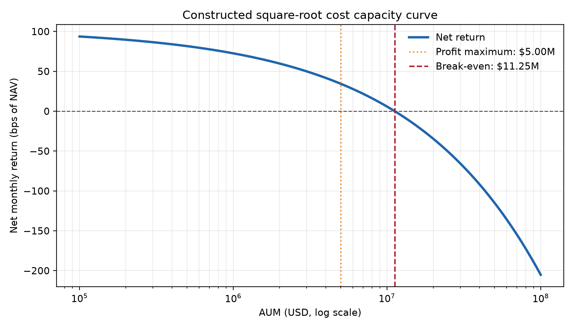
The figure fixes monthly gross excess return at 120 bps, one-sided monthly turnover at 1, 21 trading days, market ADV at USD 100 million per day, fixed unit traded-notional cost at 8.25 bps, and square-root impact coefficient at 0.05. The horizontal axis is AUM in USD on a logarithmic scale; the vertical axis is monthly net return. Under these assumptions, break-even AUM is about USD 11.248 million, and maximum net dollar return occurs at about USD 4.999 million. These values apply only to the parameters shown in the figure.

10.2 Rebalance-Cost Ablation Waterfall

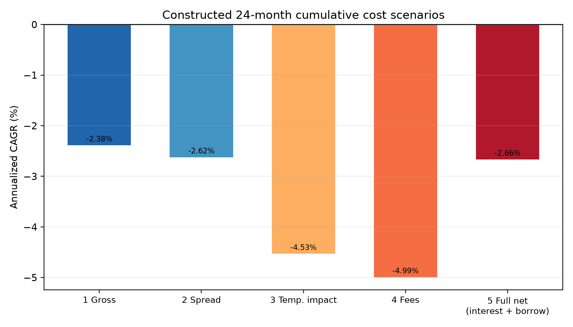
The vertical axis is annualized CAGR calculated from the staged NAV series in the 24-month constructed sample. Each bar enables one additional cost layer in a fixed order. Since the sample path, cash interest, and borrow fees interact, this is a cumulative scenario comparison; differences between adjacent bars should not be interpreted as universal causal costs for individual components.

10.3 Fix the Result Identity Before Reading the Figures

The 24-month cost-ablation figure and the original A7-B R2R6 values retain their historical constructed-path identity; they are not the result of the current signal-interface refresh dated 2026-10-14. The historical signal implementation SHA-256 is e16d97c61fea2f8cab1e7b80a6f20442232507e8b35b4bb2c1a1a2b51f0d0373; do not combine the old figure with a new results table.

The current consumer was refreshed and its scope-limited acceptance recorded by the original main controller using the original CLI/config/seed 20261210 and six fixed experiments. The entrypoint is projects/project04/cost_execution_lab/ACCEPTED_CURRENT_SIGNAL_20261014.md. The current signal implementation SHA-256 is b5357c4122116bacecb585ffe6625a7d14b9dc85c3f65c7ea1dffc744e0a4fd8, and the summary SHA-256 is 3dece7d2fd979d29c5b09b03bc19f54f508963c8e738d6fddc1e58de745e0b4e. These are all CONSTRUCTED_TEACHING_DATA.

For the current 36-period out-of-sample sample, CAGR is GROSS −1.9560%, TWAP −2.3459%, forecast VWAP −2.3327%, and lagged POV −6.0717%; corresponding Sharpes are −0.3334, −0.4014, −0.3994, and −1.0800. The high-friction negative case has full-sample net CAGR −7.4392% and Sharpe −1.5050. These negative results are retained; comparisons apply only to the same constructed path and fixed scenarios. The consumer refresh followed a correction to an exposed input implementation; it involved no new preregistration and did not calibrate real Alpha, costs, or capacity. This batch reuses that accepted summary and did not rerun the CLI or copy the complete raw CSV.

11. Real-Market Example

In institutional quantitative investing, real trading-cost structures can differ substantially from assumptions in academic models. This section summarizes cost characteristics and the limits of the current quantitative-research data using public regulatory reports and institutional empirical studies.

11.1 Findings in Institutional Empirical Literature

1. AQR study of anomaly-trading costs (Frazzini, Israel, and Moskowitz, 2012):
   • The AQR team analyzed a database of real institutional executions from 1998 to 2011, covering 19 developed markets and close to USD 1 trillion in trading.
   • The working paper reports that estimated costs for several anomaly portfolios, based on actual execution costs, were below estimates in earlier literature based on aggregated transaction or quote data. It also uses portfolio optimization to study the tradeoff between cost and tracking error and reports differences across styles.
   • These are results for that institution's sample, period, and portfolio designs. Its impact parameters cannot be generalized as universal constants, and the paper does not establish that every quantitative strategy retains significant returns after costs.
2. U.S. SEC Staff Report on Algorithmic Trading (2020):
   • The report describes core algorithmic-trading processes in U.S. equities, liquidity provision by automated market makers, and order routing in a multi-venue market.
   • It summarizes improvements in several market-quality and liquidity-provision measures under normal conditions and notes that some algorithm types may amplify risk during unusual stress or volatility. It also describes the market's multi-venue, automated structure. This chapter does not extrapolate the report into a general empirical claim about spread or depth differences between large-cap and micro-cap stocks.
3. SEC request for comment on mutual-fund transaction-cost disclosure (2003):
   • In this historical request for comment, the SEC said that there was then no universally accepted method for calculating portfolio implementation shortfall. It compared measurement approaches and requested comments on specific algorithms, formulas, and the treatment of opportunity cost. This 2003 concept paper does not establish a current universal regulatory formula. Researchers should state and freeze the benchmark used in their experiment.

11.2 Data Available in the Current Teaching Environment and Known Gaps

The inventory in qa/a7/ch35_ch36_batch/SOURCE_DATA_GAP.md defines the data boundaries for the current course stage:

• Available data: The local environment contains monthly industry and factor-return snapshots from Kenneth French (used for macro and broad asset-pricing demonstrations) and constructed monthly signals from the Project 4 preparation layer.
• Missing real-world materials: The local environment does not have per-stock intraday Level 2/Level 3 order-book replay data, daily historical intraday stock-borrow rates and availability flags, or live execution records containing broker dark-pool and smart-routing fills.
• Boundary: All friction parameters in this chapter, examples, and later experiments—including impact coefficients $\lambda_{\text{impact}}$, participation caps, and borrow rates—are carefully designed teaching inputs. Readers should learn the internally consistent cost model and ledger reconciliation method, but must not treat these constructed inputs as production-market calibrations or infer evidence of a real, profitable Alpha.

12. Common Mistakes

Four trading-cost errors commonly arise in quantitative engineering and strategy research.

Mistake 1: Double-Charging Frictions Embedded in the Fill Price as Cash Fees

What goes wrong: A backtest matching engine first adjusts the fill price $P^{\text{fill}}$ for spread and impact, then deducts the spread and slippage again as separate cash fees.

Incorrect code:

# Incorrect: double charging
fill_price = mid_price + 0.5 * spread + impact  # The buy price already includes the increase.
# Deduct the purchase payment.
cash -= qty * fill_price
# Error: deduct the half-spread and impact loss again!
cash -= qty * (0.5 * spread + impact)

Consequence and numerical error: For a trade buying 10,000 shares at a midpoint of USD 100, with a half-spread of USD 0.05 and temporary impact of USD 0.10, the actual fill price is USD 100.15. The payment is USD 1,001,500, including USD 1,500 of friction. The incorrect code over-debits cash by USD 1,500, doubles the modeled trading friction, and may falsely eliminate a strategy that would otherwise be profitable.

Correct repair:

# Correct ledger entry: the fill price absorbs friction; deduct explicit fees separately.
fill_price = mid_price + 0.5 * spread + impact
cash -= (qty * fill_price + explicit_commission)

Mistake 2: Multiplying by 2 Again After Total Traded Notional Already Includes Both Sides

What goes wrong: Let one-sided turnover be $\tau_{\text{turnover}}=\frac12\sum_i|w_i^*-w_i^-|$. If total traded notional is first computed as $V_{\text{trade}}=2\tau_{\text{turnover}}\,\text{NAV}$, it already includes both buys and sells. Multiplying $2V_{\text{trade}}$ by the cost rate per dollar traded double counts total notional. If $V_{\text{trade}}$ was instead computed directly from the two-sided weight change $\sum_i|w_i^*-w_i^-|$, it must not be multiplied by 2 again either.

Incorrect and corrected forms:

# Incorrect: total_notional already includes both buy and sell notional.
total_notional = np.sum(np.abs(target_weights - current_weights)) * portfolio_nav
# Incorrect: cost_total = 2.0 * total_notional * single_trip_fee_rate
# Correct:
one_sided_turnover = 0.5 * np.sum(np.abs(target_weights - current_weights))
# Total cost, using a rate per dollar traded:
cost_total = total_notional * single_trip_fee_rate
# Equivalently, start from one-sided turnover and multiply by 2 only once:
cost_from_one_sided = (2.0 * one_sided_turnover) * portfolio_nav * single_trip_fee_rate

Mistake 3: Charging Full Commission on Unfilled or Partially Filled Orders

What goes wrong: In the ledger model used here, a limit order with no fill ($F=0$, $R=Q$) is incorrectly charged broker commission and stamp tax based on the parent-order quantity $Q$.

Consequence and repair: In this model, explicit fill commission is tied to actual executed quantity $F$. The unfilled remainder $R$ contributes opportunity-cost attribution in implementation shortfall; it is not charged the modeled fill commission in the cash ledger. Other account-specific order-submission or cancellation fees are outside this model.

# Correct repair
actual_commission = commission_per_share * abs(filled_qty)  # Use filled_qty, not parent_qty.

Mistake 4: Setting Fill VWAP to Zero When There Are No Fills, Which Breaks Return Calculations

What goes wrong: When a stock is limit-up for the day or liquidity dries up and the fill quantity is zero, the code defaults fill_vwap to 0.0.

Consequence and repair: If fill_vwap = 0.0, later calculations of slippage or return from the fill price produce the nonsensical result $(0.0-P_{\text{arrival}})/P_{\text{arrival}}=-100\%$, resembling a catastrophic loss.

# Correct repair: with no fills, VWAP must be None or np.nan.
fill_vwap = (total_fill_notional / total_filled_qty) if total_filled_qty > 0 else np.nan

13. Quantitative-Research Applications

In quantitative research, transaction costs should not be added as an after-the-fact patch. They belong as an ex ante constraint embedded directly in the portfolio-optimization objective.

13.1 Cost-Aware Portfolio Optimization

A conventional mean-variance optimizer maximizes expected return while penalizing risk:

Here $\lambda_{\text{risk}}$ applies to returns and return variance at the same frequency and is a local tradeoff parameter in a return objective. It differs from the USD$^{-1}$ parameter required by Chapter 36's dollar-IS objective; the numerical values cannot be reused across those objectives.

This frictionless optimizer can induce frequent small weight changes and generate turnover whose marginal return is below its trading cost. A cost-aware optimizer places trading costs directly in its objective:

If $\text{Cost}_i$ is in dollars, divide by NAV before subtracting it from the dimensionless return objective. Write cost as $c_i|\Delta w_i|+\kappa_i(\Delta w_i)^2$. Sufficient conditions for a convex QP are fixed $\text{NAV}>0$, a symmetric positive semidefinite covariance matrix $\Sigma$ at the same frequency, $\lambda_{\text{risk}}\ge0$, dollar cost coefficients $c_i\ge0$ and $\kappa_i\ge0$, and linear portfolio constraints. Introduce $u_i\ge\Delta w_i$ and $u_i\ge-\Delta w_i$, replacing the absolute-value penalty in the maximization objective by $-c_i u_i/\text{NAV}$. This gives an equivalent convex quadratic program (QP). If $c_i>0$, the penalty makes $u_i=|\Delta w_i|$ at an optimum; if $c_i=0$, $u_i$ may be slack without changing that term or the optimal objective value. Nonnegativity matters: with $\Delta w=0$, $c=-1$, $\text{NAV}=1$, and zero return and risk terms, the original objective is 0, whereas the relaxed problem becomes unbounded as $u\to\infty$.