Time Series I: Dependence and ARIMA

Roadmap: First explain how a series depends on its past over time, then estimate a model that uses only past information and evaluate it with forecasts that advance strictly in time.
Prerequisites: Chapters 6 on probability, 7 on statistics, 8 on regression, and 11 on returns and performance measures. By the end, you will be able to distinguish price levels from returns; define weak and strict stationarity; explain the difference between white noise and IID; calculate the mean, variance, and autocorrelation of an AR(1) by hand; read ACF/PACF plots; compare AR, MA, ARMA, and ARIMA models; diagnose residuals; calculate prediction intervals; and write a month-by-month expanding-window forecast.

1. Learning Objectives

By the end of this chapter, you should be able to do five things:

1. Treat a time index with a stated frequency as part of the data; identify missing months, unsorted observations, and missing values; and refuse to compress time into row numbers with no gaps.
2. State weak-stationarity conditions from finite means, variances, and autocovariances, and explain how they relate to strict stationarity, white noise, and independent and identically distributed observations.
3. Derive the stationary mean, variance, autocovariance, ACF, and multi-step forecast-error variance from the recursion $X_t=c+\phi X_{t-1}+\varepsilon_t$.
4. Use the lag operator to explain AR, MA, ARMA, and ARIMA models; understand that ACF/PACF patterns are clues for candidate models, not automatic model selectors.
5. Restrict model-order and parameter choices to the training window, use only observations available before each forecast origin, and compare forecasts with a naive benchmark.

State mathematical units consistently: monthly returns are decimals, so 0.01 means a 1% return for that month; means and forecasts are also in monthly-return decimals; variances are in squared return decimals; ACF and PACF are dimensionless; and lag $k$ means $k$ observed months back, not $k$ calendar days of equal length.

2. Why Quants Need This

A time-series model turns the question “Does the recent value contain information about the next period?” into a question that can be stated and tested. In quantitative work, this often comes after data cleaning and before regression or strategy testing: first choose the target variable (a price, return, spread, or volatility proxy), describe how it depends on its own history, and then ask whether that relationship would have been available at the forecast time.

Storing daily, monthly, or quarterly data as a column of numbers discards the spacing between observations. If an asset has no observation for March 2024, applying dropna() and treating February and April as adjacent steps no longer makes an AR(1) a “one-month lag.” Modeling a cumulative price level as though it were a stationary return can make a trend look like strong correlation. If you choose an order using the full data and then call the second half an out-of-sample forecast, the future has already influenced the research decision.

The chapter follows a complete chain: define the observation clock → calculate autocovariance and correlation → represent dependence with a low-order model → estimate from training data → inspect what the model leaves behind → forecast forward one period at a time → compare with a naive benchmark. The time index is not decoration; it determines the meaning of a lag and the forecast target.

3. Intuition

Imagine two “monthly-return machines.” Both have a long-run average monthly return of 0.5% and a long-run one-month standard deviation of 4%. The first draws a new independent card each month. The second carries forward 70% of the previous month's deviation from its long-run mean. Their averages and volatility alone do not distinguish them; if the second machine was above average last month, it is more likely to be above average this month too. The difference lies in the ordering over time.

This kind of “memory” is described by autocorrelation. Positive lag-1 autocorrelation means neighboring months usually deviate from the mean in the same direction; a negative value means they tend to move in opposite directions. A value near zero says only that linear correlation is small; it does not rule out nonlinear dependence, volatility clustering, or common external shocks.

A common misconception is that a return series that fluctuates smoothly around a level proves that its data-generating process is stationary. A structural break, a few extreme months, or a slow stochastic trend can all mislead a finite-sample plot. A plot raises a question; theoretical assumptions and later tests provide different kinds of evidence.

3.1 A Stochastic Process Is Not a Single Line

A stochastic process is a time-indexed family of random variables $\{X_t\}$: before observation, a different return could occur in each month. A realization is one set of values actually drawn from that family, $x_1,\ldots,x_n$. The three possible worlds below distinguish “across time” from “across worlds.” This table identifies the objects; it is not a stationarity test.

The January column corresponds to the random variable $X_1$; row A is one realization. $\mathbb E[X_1]$ weights the possible worlds, while the sample mean $\bar x$ averages along the observed path; these are different operations. Estimating population moments from a long path also requires suitable ergodicity or law-of-large-numbers conditions; stationarity alone does not ensure them. For example, first draw a $Z$ and then set $X_t=Z$ for every month. This process is strictly stationary, but the mean of any long path remains the draw $Z$ and does not automatically become $\mathbb E[Z]$. Financial data usually provide only one historical path, so whether moments look stable within a window is an evidential question that cannot be settled by the line's appearance.

The population parameters of the two return machines can be written in one table. Let $s=0.04$ and $\mu=0.005$, and use a stationary initialization for the AR machine:

Equal marginal means and variances do not determine how neighboring months move together. The AR machine needs a smaller innovation variance because past shocks also contribute to the current month's total variation. Sample values in a finite data table will not exactly match these population parameters.

4. Mathematical Foundations

Let $X_t$ be a random variable indexed by month; $t$ denotes the position of a monthly observation, and $X_{t-k}$ is $k$ observed months earlier. If $P_t$ is the month-end price, the simple and log returns are, respectively:

If prices are quoted in euros, $P_t$ is measured in euros per share, while returns $R_t$ and $r_t$ are dimensionless. For small returns, $r_t\approx R_t$, but they differ for larger moves. A price level, a simple return, and a log return are three different series; a model must state which one it forecasts.

This chapter represents calendar months with a monthly PeriodIndex. The lag from 2024-02 to 2024-03 is one month even when the two calendar months have different numbers of days; this does not assume February and March have the same number of days. A missing month is a missing observation, not an excuse to treat “the next CSV row that remains” as a one-month lag. The core code requires consecutive months and rejects NaN, positive or negative infinity, and complex inputs; it does not fill values automatically.

For a stationary series with finite variance, its mean, variance, and autocovariance are:

Here, $\mu$ has the same units as $X_t$; $\gamma(k)$ has units equal to the square of the variable's units; $\rho(k)$ is dimensionless, and $\rho(0)=1$. If $X_t$ is a monthly return, $k=12$ means 12 observed months apart; it does not automatically mean 365 days or any fixed number of calendar days.

5. Formal Definitions

Strict stationarity requires that, for every positive integer $m$, every set of observation positions $t_1,\ldots,t_m$, and every common shift $h$, the vectors $(X_{t_1},\ldots,X_{t_m})$ and $(X_{t_1+h},\ldots,X_{t_m+h})$ have the same joint distribution. It compares the full distribution and dependence structure, not only the mean and variance.

Weak stationarity (also called covariance stationarity) requires finite second moments, a mean that does not vary with $t$, and an autocovariance $\operatorname{Cov}(X_t,X_{t-k})$ that depends only on the separation $k$, not on the calendar starting point $t$. Strict stationarity with finite second moments implies weak stationarity; the converse generally fails. An exercise in Section 18 constructs a counterexample from independent series with different marginal distributions but identical first two moments.

White noise (WN) uses a second-order definition in this chapter: $\mathbb{E}[\varepsilon_t]=0$, $\operatorname{Var}(\varepsilon_t)=\sigma^2<\infty$, and zero autocovariance at every nonzero lag. White-noise observations need not be independent. Independent and identically distributed (IID) additionally requires independence across periods and the same marginal distribution. Zero-mean, finite-variance IID noise is white noise; “correlations close to zero” do not imply IID. If the noise is jointly Gaussian, zero correlation does imply independence.

The autocorrelation function (ACF) lists how $\rho(k)$ changes with lag $k$. The sample ACF divides sample autocovariance by sample variance; different denominator conventions across software can produce small finite-sample differences. The partial autocorrelation function (PACF), after controlling for the intermediate lags $X_{t-1},\ldots,X_{t-k+1}$, measures the remaining linear relationship between $X_t$ and $X_{t-k}$. It can also be viewed as the coefficient on the farthest lag in the linear projection for $\mathrm{AR}(k)$.

For observations $x_1,\ldots,x_n$, a common sample definition is:

Here $n$ is the number of sample months, $k$ is the lag in months, and $\bar x$ is the sample mean. Using $n$ or $n-k$ in the denominator gives different finite-sample estimates; the code in this chapter explicitly uses the former convention. The PACF can also be defined by linearly projecting $x_t$ on all variables from lag 1 through lag $k$ and reading the population projection coefficient on the final term $x_{t-k}$; finite-sample estimators can differ.

An autoregressive model ($\mathrm{AR}(p)$) writes the current value as a finite sum of its own lags and an innovation. A moving-average model ($\mathrm{MA}(q)$) writes the current value as a linear combination of the current and previous $q$ innovations. An autoregressive moving-average model ($\mathrm{ARMA}(p,q)$) contains both structures. An autoregressive integrated moving-average model ($\mathrm{ARIMA}(p,d,q)$) first differences the series $d$ times and then describes the differenced process with an ARMA model.

The lag operator $L$ is defined by $LX_t=X_{t-1}$, so $L^kX_t=X_{t-k}$. Lag polynomials write finite-lag equations compactly. A process has a stable causal stationary solution when all roots of its AR polynomial lie outside the unit circle; a model is invertible when all roots of its MA polynomial lie outside the unit circle. For the AR(1) and MA(1) models here, these conditions reduce to $|\phi|<1$ and $|\theta|<1$, respectively. Polynomial sign conventions vary, so check the definition before using software.

A prediction interval, conditional on a model and information set, gives an uncertainty range for one future observation. It is wider than a confidence interval for the conditional mean because the future innovation also varies. With normal errors, parameters treated as known, and forecast variance $V_h$, a common form is:

Here $\hat X_{T+h\mid T}$ has the same units as the series, $V_h$ is the forecast-error variance for the future observation, and $z_{1-\alpha/2}$ is a standard-normal quantile. Estimated model parameters, heavy-tailed innovations, conditional heteroskedasticity, and structural changes affect interval coverage; an interval is not a guarantee.

6. Derivations

6.1 AR(1): From the Recursion to Stationary Moments

Start with an AR(1) with an intercept:

$c$ has the same units as $X_t$, $\phi$ is dimensionless, and $\varepsilon_t$ has the same units as $X_t$. Assume the innovation has mean zero and variance $\sigma^2$, and is uncorrelated with the past. If a stable stationary solution exists, take expectations:

Under the causal stationarity condition $|\phi|<1$, the long-run mean is the expression above. Define the centered variable $Y_t=X_t-\mu$ and substitute it into the recursion to obtain:

Centering separates the long-run level from variation around it; here $\mathbb{E}[Y_t]=0$. Using the fact that the innovation is uncorrelated with the previous value $Y_{t-1}$, square the equation and take expectations:

In the causal setup used here, the innovation is a new shock in the current period and is uncorrelated with the past. For the shock weights $1,\phi,\phi^2,\ldots$ to decay and the causal representation to converge, we must have $|\phi|<1$. Rearranging the variance equation formally gives $\sigma^2/(1-\phi^2)$, but when $|\phi|\ge1$ it no longer yields a finite, nonnegative causal stationary variance. This chapter discusses causal AR(1); other noncausal representations are out of scope.

Next, multiply $Y_t=\phi Y_{t-1}+\varepsilon_t$ by $Y_{t-k}$ and take expectations. For $k\ge1$, the current innovation is uncorrelated with the past value $Y_{t-k}$, so:

Repeated application of the recursion gives $\gamma(k)=\phi^k\gamma(0)$, and therefore:

If $\phi=0.7$, the autocorrelation decays as $0.7,0.49,0.343,\ldots$; if $\phi<0$, its sign alternates each period; if $\phi$ is close to 1, decay is slow and a finite-sample plot may look highly persistent. Slow decay in a finite plot does not by itself prove a unit root; unit-root tests and correlated common trends are covered in Chapter 17.

When $|\phi|<1$, repeated substitution writes the centered series as:

The remainder after a finite expansion is $\phi^mY_{t-m}$, which vanishes as $m$ increases for a stable causal solution with finite variance. This shows that the current value is a weighted sum of recent shocks, with old-shock weights shrinking as $\phi^j$. If the innovations are IID, this causal representation also helps establish strict stationarity. Second moments under white-noise assumptions give the weakly stationary moments derived above, but do not establish invariance of every joint distribution.

6.1.1 A Stable Recursion and a Stationary Initialization Are Different Things

$|\phi|<1$ means that the effect of an old state decays; if the process starts from an arbitrary fixed $X_0$, the first few periods need not have stationary moments. Iterate the recursion for $h$ periods, substituting $c=(1-\phi)\mu$ at each step, to obtain:

Assume the future innovations are independent of $X_0$, have mean zero, and are uncorrelated with one another:

The first term comes from the starting value; the second comes from innovations that have entered the process. A fixed starting value has variance zero. Let $\mu=0.005,\phi=0.5,\sigma=0.06$ and start from $X_0=\mu$:

The means are equal, but the variance changes over time, so the process initialized at the left is not weakly stationary. If $X_0$ is independent of future innovations and has mean $\mu$ and variance $\sigma^2/(1-\phi^2)$, then the second moments are stationary from the start. For strict stationarity with IID innovations, the full distribution must also be initialized from the stationary causal solution. With normal innovations, draw $X_0\sim N(\mu,\sigma^2/(1-\phi^2))$. Discarding a simulation warm-up period only makes the starting-value effect smaller; it does not make the process exactly stationary after any finite warm-up.

6.2 How Multi-Step Forecast Errors Widen

To derive the conditional forecast mean and forecast-error variance, assume that future innovations are independent and identically distributed, and that the entire set of future innovations is independent of the information available at the forecast origin; innovations have mean zero and variance $\sigma^2$. This is stronger than unconditional second-order white noise alone. Let $\mathcal F_T$ denote the information through month $T$. The one-step AR(1) forecast mean is:

The value $X_T$ on the right is known at the forecast time. The conditional mean of a future innovation is zero, so this is the “conditional mean of next month's return,” not the return that will necessarily be realized next month. For the following month, $X_{T+1}$ is still unknown, so replace it with the one-step forecast just calculated:

For an $h$-step horizon, the conditional forecast mean is $\mu+\phi^h(X_T-\mu)$. The forecast error includes future innovations:

Under these assumptions, conditional on $\mathcal F_T$, each future innovation still has conditional variance $\sigma^2$, and conditional covariances between different future periods are zero. Add the terms in the conditional forecast-error variance to obtain:

Here $V_h$ has units of squared monthly-return decimals. As $h$ increases, more future innovations are unknown; as $h\to\infty$, forecast uncertainty approaches the unconditional variance $\sigma^2/(1-\phi^2)$. This derivation treats the parameters as known; fitting a model also introduces parameter-estimation uncertainty.

How the Information Set Changes the “Best” Forecast

The conditional mean is the optimal forecast under squared-error loss, given $\mathcal F_T$. If we assume only second-order white noise, the AR recursion above still gives a linear forecast based on past values, but not necessarily the conditional mean among all measurable functions. A concrete counterexample is $U\sim\mathrm{Uniform}(0,2\pi)$, $e_t=\cos(2^tU)$ ($t=0,1,\ldots$): each period has mean zero and variance $1/2$, and cosine waves at different frequencies are orthogonal, so nonzero-lag autocovariances are zero; nevertheless:

Given the past value $e_t$, the next value is fully known, and $\mathbb E[e_{t+1}\mid e_t]=2e_t^2-1$ is generally not zero. Second-order white noise cannot replace the assumption that the conditional mean of a future innovation, given the available information, is zero. The numerical forecasts in this chapter explicitly use the stronger independent-innovation assumption; with conditional heteroskedasticity, the conditional forecast-error variance must also be rederived.

6.3 MA(1), Invertibility, and ARMA

First distinguish two objects both called a moving average. The rolling price mean $M_t=(P_t+P_{t-1}+P_{t-2})/3$ is a smoothing indicator calculated from observed prices, measured in currency per share. The MA(1) process $X_t=\mu+\varepsilon_t+\theta\varepsilon_{t-1}$ is a data-generating model whose filter acts on innovations that cannot be observed directly. The first can be calculated from prices; the second requires identifying or estimating the model's innovations. Let the innovations (in return decimals) be $\varepsilon_{t-1}=0.02,\varepsilon_t=-0.01$ and $\theta=0.5,\mu=0.005$, with $X_t=0.005-0.01+0.5(0.02)=0.005$; this does not average the two monthly returns. The three-period rolling mean of prices $100,103,102$ is $101.6667$ currency per share.

Use the MA(1) sign convention $X_t=\mu+\varepsilon_t+\theta\varepsilon_{t-1}$. The current value combines this month's new shock with last month's shock. For the centered series, two adjacent months are, respectively, $X_t-\mu=\varepsilon_t+\theta\varepsilon_{t-1}$ and $X_{t-1}-\mu=\varepsilon_{t-1}+\theta\varepsilon_{t-2}$. If innovations have mean zero, variance $\sigma^2$, and are uncorrelated across months, then:

The lag-0 variance adds the variances of the two terms because $\varepsilon_t$ and $\varepsilon_{t-1}$ are uncorrelated. At lag 1, the two series share only $\varepsilon_{t-1}$; the product of its coefficients is $\theta$, so the covariance is $\theta\sigma^2$. At separations of at least two months, no innovation is shared, so the covariance is zero. Thus the population ACF of an MA(1) cuts off after lag 1. A finite-sample ACF will not become exactly zero; it fluctuates around the population pattern.

The theoretical ACF of an MA(1) is zero from lag 2 onward, while the PACF generally decays gradually. If $|\theta|<1$,

Because $(1+\theta L)^{-1}=1-\theta L+\theta^2L^2-\cdots$, when $|\theta|<1$ the weights on the right decay geometrically; substituting current and past values then recovers the innovations stably. This is called invertibility. An MA process is a finite linear combination of white-noise terms and is therefore stationary for finite $\theta$; noninvertibility does not mean nonstationarity. Invertibility is an identification restriction that gives an observable series a unique, stable innovation representation.

The PACF of $\mathrm{AR}(p)$ theoretically cuts off after lag $p$, while its ACF usually tails off. The ACF of $\mathrm{MA}(q)$ cuts off after lag $q$, while its PACF usually tails off. ARMA models usually have both functions tail off. These are ideal population patterns; noise, roots near the unit circle, and mixtures of model structures can blur them in finite samples. Do not choose an order only by eye from the “closest-looking” plot.

6.4 Differencing and Over-Differencing

First differencing is defined by $\Delta X_t=X_t-X_{t-1}=(1-L)X_t$. An $\mathrm{ARIMA}(p,d,q)$ model represents $\Delta^d X_t$ with an $\mathrm{ARMA}(p,q)$ model. If $X_t$ is a price, $\Delta X_t$ is a price change in currency per share; if $X_t=\log P_t$, $\Delta X_t$ is exactly the log return over that interval, and only approximates the simple return for a small change. If $X_t$ is already a return, differencing it gives a “change in returns,” not the usual holding-period return.

From input to output, first differencing subtracts last month's level from this month's level and drops the first month, which cannot be paired. For example, for month-end prices $[100,101,103,102]$ euros per share, the differenced output is $[1,2,-1]$ euros per share; this is a price change, not a percentage return. Differencing log prices instead gives an approximation to the simple return. Differencing aims to remove a shared accumulation in levels under assumptions such as a stochastic trend; it does not automatically make every series stationary, and it changes the forecast target.

Differencing can remove a stochastic trend, but it also loses the first sample row and changes the question. If the original monthly series is already white noise, $X_t=\varepsilon_t$, differencing it gives:

This is the boundary case of an MA(1) with $\theta=-1$; its variance is $2\sigma^2$, lag-1 autocovariance is $-\sigma^2$, and ACF(1) is $-1/2$. Adding a difference has instead created pronounced negative correlation, known as over-differencing. Choose $d$ only with a reason tied to the target variable and trend; Chapter 17 discusses ADF tests, deterministic trends, and unit-root identification in detail.

6.5 Returning a Differenced Forecast to the Original Quantity

If a model forecasts $D_t=\Delta X_t$, its output is still a change. From $X_{T+h}=X_T+\sum_{j=1}^{h}D_{T+j}$, take the conditional expectation using the same information set:

The last observed price is 102 euros per share, and the predicted changes for the next two months are 1 and 2 euros per share, giving level forecasts of 103 and 105. If the two change-forecast errors $v_1,v_2$ each have variance 4 and covariance 1, the second-period level error is $v_1+v_2$, with variance $4+4+2(1)=10$ euros squared per share squared. Do not simply add the endpoints of separate one-period intervals.

Log prices add another complication: if $X=\log P$, after forecasting log level $m$, $e^m$ is usually not $\mathbb E[P\mid\mathcal F_T]$. Under a conditional normal distribution with variance $V$, the conditional mean price is $e^{m+V/2}$, while $e^m$ is the conditional median. Without a specified conditional distribution, do not apply this correction mechanically. The chapter's forecast_arima returns a forecast of whichever series it receives; if the original level is passed with $d=1$, statsmodels has already transformed the forecast back to levels internally, so do not cumulate it again.

6.6 How Long Is One Lag?

The population ACF/PACF objects were defined in Section 5; sample estimates suggest candidates, while out-of-sample errors show how a candidate forecasts the next period. Both depend on a valid observation clock: month labels use calendar time, trading-day numbers use trading time, and transaction numbers use event time. One step of a transaction-level AR(1) means the next transaction, which may occur milliseconds or hours later; it is not automatically a one-minute forecast. For a one-minute forecast, first define a one-minute grid and specify what a no-trade interval means.

In the missing-month example, February to April is two steps. Given the February state, the April conditional-mean deviation in the same AR(1) model is multiplied by $\phi^2$, and the error variance is $\sigma^2(1+\phi^2)$. Using $\phi$ and $\sigma^2$ as though the rows were adjacent gets both the target and the risk wrong. The monthly interface in this chapter stops when it finds a gap; it does not fill months or choose a new clock for the researcher.

7. Financial Interpretation

When modeling an asset price $P_t$, a long-run upward trend can make $P_t$ and $P_{t-1}$ highly correlated even when the tradable return $R_t$ is not predictable. High ACF in a price level cannot be translated directly into “next month's return is predictable.” First define the return interval, then state whether the target is a month-end-to-month-end simple return, log return, or another contractual return.

If monthly returns follow a stable AR(1), a positive $\phi$ means that returns recently above the mean partly persist in the model; a negative $\phi$ means linear reversal in the model. This describes time dependence only. An estimate could reflect market microstructure, nonsynchronous trading, dividend-reinvestment conventions, crisis-regime shifts, or sample selection. The univariate model in this chapter explains no causal mechanism and says nothing about trading costs, borrow availability, or capacity.

Linear return autocorrelation and volatility clustering are separate issues. Even when the return ACF is near zero, $|R_t|$ or $R_t^2$ may remain persistent; the white-noise condition describes only second-order linear correlation in the series. This chapter develops ARMA tools mainly for the conditional mean; conditional-heteroskedasticity models are left to later chapters. Failure to reject the null of no residual linear autocorrelation with Ljung–Box does not prove that residuals are IID, normal, or homoskedastic.

Tradable timing cannot be inferred from a month label alone. If $R_t$ is the return from the end of March to the end of April, the April return is not fully observable until that interval ends; using it to forecast “the April return” reverses time. A research design must specify data available_at, signal signal_time, the earliest executable trade_time, and the target return interval. French monthly portfolio files do not report historical release times month by month, so they describe the published historical series but do not provide a point-in-time training set.

8. Numerical Example

Now consider an MA(1) with $\theta=0.5,\sigma=0.06$. Then $\gamma(0)=0.0036(1+0.25)=0.0045$ and $\gamma(1)=0.5(0.0036)=0.0018$, so $\rho(1)=0.4$, while $\rho(k)=0$ for every $k\ge2$. Its ACF shape differs from that of an AR(1), although both can explain correlation between adjacent periods.

Finally, compare the two constructed return machines with common mean 0.005 and marginal standard deviation 0.04. Every nonzero-lag population ACF of the IID machine is zero. Set the AR(1) machine to $\phi=0.7$; its innovation standard deviation should then be $0.04\sqrt{1-0.7^2}\approx0.02857$, and its population ACF(1) is 0.7. This adjustment gives both machines the same theoretical unconditional variance, $0.04^2$, without forcing their finite-sample variances to match exactly.

9. Python Implementation

Default Entry Point for This Reader Edition

From the accepted I3 reader package root, create an independent environment using its environment instructions, then run:

.venv/bin/python run_notebook.py notebooks/ch16_time_series.ipynb

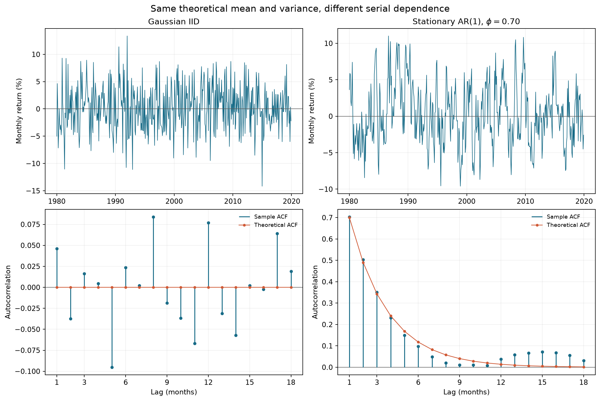
With seed 20261016, the default run constructs 480 months of IID and AR(1) returns from 1980-01, with mean 0.005, marginal standard deviation 0.04, and AR coefficient 0.7. The AR starting value is drawn from its stationary normal distribution; the innovation standard deviation is 0.04 times sqrt(1−0.7²). It checks theoretical moments and sample ACF/PACF, then trains on the first 360 months through 2009-12 and forecasts three months starting in 2010-01. Training residuals receive a Ljung–Box check with lag=12 and model_df=1. Over the final 120 months, expanding-window one-step ARIMA forecasts are compared with the mean available from each training window using RMSE.

The Notebook displays the existing bundled figure fixtures/figures/a4/ch16_stationarity_acf.png; displaying it does not regenerate it. RUN_FRENCH=False disables the historical market branch. Although it creates and prints runs/ch16_time_series_<uuid>/, this Notebook writes no CSV or PNG there. The runner separately saves the executed copy and status in a unique runs/execution_* directory; these directories serve different purposes. Constructed calculations are not evidence of market predictability or strategy net returns. The historical French figures and numbers in Sections 10–11 retain their original status.

The CLI and production tests below belong to the historical course working-root workflow and are not this package's default route. Readers need not restore production tests that are absent from the package. The I3 Chapter 16 CLI still reads French data unconditionally; the Chapter 17 CLI's historical branch requires --french-data. Neither replaces the default command above.

Historical Course Working Root and Original Implementation

The core implementation for this chapter is in time_series.py. validate_monthly_series requires a sorted, unique, consecutive PeriodIndex(freq="M") with finite real values; it explicitly rejects missing months, NaN, infinity, and complex numbers. split_monthly_series splits by row count into earlier and later observations without shuffling. forecast_arima(train, ...) receives only the training prefix; rolling_origin_forecast refits an expanding window before each target month and forecasts the next month. This teaching wrapper supports only nonseasonal differencing orders $d=0$ or 1; it does not include exogenous regressors, seasonal terms, or complex missing-state estimation.

The statsmodels ARIMA likelihood implementation may issue numerical-convergence warnings for very small decimal returns. The fitting function in this chapter multiplies monthly return decimals by 100 to fit in percentage points, then scales forecast means, intervals, and residuals back to decimals; AR/MA coefficients do not change under this uniform linear scaling. FittedARIMA.result is the fitted statsmodels result in percentage-point units. Its intercept, residuals, and innovation standard deviation remain in percentage points if read directly; use .residuals to obtain residuals in decimals.

For estimation, the input is a monthly-return series ending at the forecast origin, and the model order $(p,d,q)$ must be specified first. fit() estimates parameters on that training sample; only then does get_forecast() produce future conditional means and prediction intervals. ACF/PACF help narrow the candidates. AIC/BIC can compare fitted candidates within the training window, followed by MAE/RMSE comparisons on a time-ordered validation window; the final holdout must not be used for repeated order selection.

For $d=0$, this wrapper uses trend="c". Statsmodels treats the trend term as a regression constant, so const here denotes the constant level or unconditional mean of the series. In the textbook recursion with intercept $X_t=c+\phi X_{t-1}+\varepsilon_t$, the two constants satisfy $c=(1-\phi)\mu$; do not treat the fitted const as the recursion's $c$. For $d=1$, the wrapper uses trend="n", with no drift term estimated. The model also constrains AR roots to be stationary and MA roots to be invertible, and it raises an error for missing values. These computational settings do not prove that the data satisfy the model. Standard prediction intervals depend on the innovation structure; normal intervals also depend on a normal-error approximation, and parameter uncertainty is not automatically included when parameters have been estimated.

From the quant_course/ project root, run the script and the focused tests:

.venv/bin/python code/ch16_time_series.py
.venv/bin/python -m pytest -q tests/test_ch16_time_series.py

The script uses fixed seed 20261016 to generate 480 months of constructed IID and AR(1) data, plots them, prints theoretical and sample moments and expanding-window simulation RMSE, and reads the French industry snapshot for descriptive statistics. The notebook ch16_time_series.ipynb must be rerun from its first cell using the quant-course-venv kernel. The notebook calls src/ directly rather than reimplementing the core functions.

The following is a complete monthly split and one-step forecast example. Return decimals represent monthly returns; target_period is the target month of a forecast, not the actual trade_time.

import numpy as np

from quant_course.time_series import (
    forecast_arima,
    simulate_stationary_pair,
    split_monthly_series,
    training_mean_forecast,
)

monthly_returns = simulate_stationary_pair(
    n=120, seed=20261016, mean=0.005, marginal_sd=0.04, phi=0.7
)["ar1"]
train, test = split_monthly_series(monthly_returns, train_size=96)
prediction = forecast_arima(train, steps=1, order=(1, 0, 0))
baseline = training_mean_forecast(train, steps=1)
print("train through:", train.index[-1], "target:", prediction.index[0])
print("ARIMA forecast:", float(prediction.iloc[0]["forecast"]))
print("training-mean baseline:", float(baseline.iloc[0]))
print("realized test return, for retrospective scoring only:", float(test.iloc[0]))
assert prediction.index[0] == test.index[0]
assert np.isfinite(prediction.to_numpy()).all()

For sample ACF/PACF, sample_acf_pacf explicitly returns lags 1 through $L$, excluding lag 0. It uses statsmodels' ACF settings adjusted=False, fft=False, missing="raise" and PACF setting method="ywadjusted". Finite-sample ACF/PACF confidence bounds depend on additional assumptions; crossing a line in the chapter's plot is not treated as proof of a model.

10. Visualization

The figure below shows 480 months of simulated data generated by the script with seed 20261016. The top row has monthly observation time on the horizontal axis and monthly return in percentage points on the vertical axis. The bottom row has lag in months horizontally and dimensionless ACF vertically. Blue shows the sample ACF; orange shows the population ACF implied by the generating parameters. The IID process has an orange line at zero, while the AR(1) population correlation decays as $0.7^k$. The blue line does not match the population curve at every lag because this is a finite sample. The figure contains no market returns, forecast returns, or strategy performance.

11. Real Market Example

The local real-data sample is the current monthly value-weighted return cache for the French 10 industry portfolios, monthly industry-return CSV, with the original source at the data details page and the saved data manifest. The cache was parsed from a ZIP downloaded on 2026-10-05, selecting the “Average Value Weighted Returns — Monthly” block and dividing source percentages by 100. It contains 1,202 months, from 1926-07 through 2026-08. These are published industry-portfolio returns, not single-stock OHLCV prices or fund execution returns.

The script reads the NoDur column (consumer nondurables) and obtains a mean of 0.009411, sample standard deviation 0.045564, sample ACF(1)=0.094385, and ACF(12)=0.034820. These numbers confirm that the fields, units, and descriptive calculations ran; they do not show significance, stability, predictable returns, or strategy effectiveness. Monthly returns are not a sample whose homoskedastic IID properties are guaranteed by construction. The A1 manifest also says this cache is the current published version and cannot reconstruct the version visible in each historical month, so it cannot support a claim of a genuine historical rolling forecast.

The parsing rule preserves month as a YYYYMM string and then converts it to PeriodIndex(freq="M"); every industry column contains simple monthly returns in decimals. The data have no daily OHLCV block, so they cannot be converted into daily observations. The manifest has not verified a general license for redistribution outside the course; public download does not automatically permit unrestricted forwarding.

12. Common Mistakes

Treating month-end DatetimeIndex values as equally spaced days. February 29 to March 31 and March 31 to April 30 are both one observation month even though the number of calendar days differs. Use a monthly PeriodIndex for monthly series. If the task depends on actual days or business days, explicitly define a different time scale instead of guessing from row numbers.

Dropping missing months before calculating lags. Applying dropna() makes the remaining rows adjacent, so the model cannot see that the observations are two months apart. This chapter rejects gaps and missing values. To address one, return to the source, determine what the missingness means, and define an appropriate method; do not automatically fill with zero, forward-fill, or pretend the observations are equally spaced.

import numpy as np
import pandas as pd

from quant_course.time_series import validate_monthly_series

incomplete = pd.Series(
    [0.01, -0.02],
    index=pd.PeriodIndex(["2024-01", "2024-03"], freq="M"),
    name="monthly_return",
)
try:
    validate_monthly_series(incomplete)
except ValueError as error:
    print(type(error).__name__ + ":", error)

Confusing price levels with returns. For prices 100, 110, and 121, the price autocorrelation is usually high because the previous price enters the current price directly, while the simple returns are 10% and 10%. Even a good AR(1) fit to prices does not show that returns have the same predictive relationship. When needed, calculate returns for the stated research target and define the return interval separately.

Choosing an order because the ACF/PACF “cuts off.” Sample correlations are estimates, and random spikes are likely somewhere among dozens of lags. A low-order plot pattern only suggests candidates. Select orders within the training window, then compare forecast loss on a time-ordered validation window. Do not repeatedly change $p,q,d$ while looking at the final holdout.

Choosing transformations or estimating preprocessing on the full sample before splitting. A fixed causal backward difference, applied only to observations available at each origin, does not by itself use future information. Leakage can arise when full-sample decisions choose whether or how to transform, fit an estimated preprocessing step, impute values, or otherwise bring future information into past modeling decisions. Define the raw data with its availability times first; align training and validation cutoffs with forecast origins; fit each estimated transformation using training data only.

Calling a large Ljung–Box p-value “independent residuals.” The test checks a set of linear autocorrelations for a selected lag set and asymptotic reference distribution. Small-sample power is limited, and it does not check autocorrelation in squared residuals, heavy tails, or parameter stability. Report the test's $H_0$, lags, model degrees of freedom, sample size, and residual plots, then state a bounded conclusion.

Starting from residual sample $e_1,\ldots,e_n$, calculate sample autocorrelations for lags $1$ through $h$, then combine them as follows:

The null hypothesis is that the population residual autocorrelations at these lags are jointly zero. Under the usual asymptotic calibration, the reference degrees of freedom are $h-m$, where $m$ denotes model_df (for an ARMA fit, this usually subtracts the number of estimated AR and MA parameters). For example, when $h=12,m=1$, use 11 degrees of freedom. A small p-value suggests remaining linear structure; a large p-value only means this test did not provide enough evidence to reject the null.

import pandas as pd

from quant_course.time_series import ljung_box_diagnostic, simulate_stationary_pair

residuals = simulate_stationary_pair(n=120, seed=20261016)["iid"]
diagnostic = ljung_box_diagnostic(residuals, model_df=1, lag=12)
print(diagnostic.to_string())
print("Interpretation: a failure to reject is not proof of IID residuals.")

13. Quant Research Application

First narrow the research question to: “Do past monthly returns improve the point forecast for next month's return?” This is neither “Does AR(1) prove a causal momentum mechanism?” nor “Can we trade at no cost?” A complete design can follow these steps:

1. Define the variable and clock. Record the source, currency, frequency, adjustment/dividend convention, and monthly interval for the price or portfolio return. If a feature $X_t$ uses data that are not complete until the end of month $t$, its available_at cannot precede the actual release time. Set signal_time only after all inputs are visible; trade_time must follow the signal and comply with the selected market's execution rules. Define target $Y_{t+1}$ as the next month's return interval, not the same-period $Y_t$.
2. Describe the data; do not infer stationarity from a plot. Inspect separate plots of price levels and returns, missing months, outliers, distributions, and ACF/PACF. One step in a monthly PeriodIndex is one month; empirical returns are not necessarily stationary. This chapter does not perform unit-root or cointegration tests; those are covered in Chapter 17.
3. Set training and validation windows in advance. For example, train on the first 15 years and forecast one month at a time afterward; at each origin, refit parameters using only observations available before that origin. Choose orders and bandwidths within the training range and reserve the final period for one final validation. If the input source has no verifiable historical release time or version, downgrade the result to “descriptive analysis of the current snapshot”; do not call it a point-in-time backtest.
4. Compare with naive benchmarks. For returns near zero, the training mean or a zero-return forecast are clear candidates. At each origin, calculate the training mean using only earlier observations. Compute MAE/RMSE in target-return decimals and compare errors for the same forecast months. Retain the result if ARIMA does not consistently beat the benchmark.
5. Diagnose and seek disconfirming evidence. Check residual linear autocorrelation, distributional anomalies, parameter changes across windows, and errors across volatility regimes. Test sensitivity to prespecified model orders and forecast origins. If signal timing is invalid, forecast error does not beat the benchmark, improvement appears only in one period, or residuals/parameters show model failure, do not package correlation as predictable alpha.

At each step, the rolling function receives only the prefix observed earlier. It demonstrates data-access rules; it does not construct historical available_at or execute trades for you. The current French monthly-return snapshot lacks month-by-month historical ingestion/release times and therefore cannot support a valid historical point-in-time forecast experiment.

14. Chapter Summary

Define the time step, return target, and index first; only then does a lag have economic meaning. Stationarity describes whether distributional or moment structure changes over time; white noise describes second-order correlation; ACF/PACF summarize linear relationships across lags. AR, MA, ARMA, and ARIMA models parameterize these relationships but do not automatically identify an economic mechanism.

AR(1) shows the chapter's central chain: $|\phi|<1$ makes shock weights decay, giving the finite unconditional variance $\sigma^2/(1-\phi^2)$ and geometrically decaying ACF $\phi^k$. The same recursion also gives forecasts that move toward the long-run mean and forecast-error intervals that widen with the horizon. After estimation, still check residuals and out-of-sample forecasts, and keep every input within the information set available at its forecast origin.

15. Exercises

All questions are answered in Section 18 of this chapter. Unless stated otherwise, $\varepsilon_t$ denotes a zero-mean, finite-variance innovation. Hand calculations should show units and the key intermediate steps.

16-E01 (Concept). Distinguish strict and weak stationarity mathematically. Explain why strict stationarity implies weak stationarity when second moments are finite, then outline a construction that is weakly but not strictly stationary.

16-E02 (Concept). Is “white noise is IID” correct? Construct a process with mean zero, variance 1, zero autocovariance at every nonzero lag, and dependence; identify observable evidence of the dependence.

16-E03 (Concept). How do the typical population ACF/PACF patterns help distinguish AR(1), MA(1), and ARMA(1,1)? Explain why these patterns alone cannot determine the order.

16-E04 (Time axis). A CSV contains three monthly returns dated 2024-01, 2024-02, 2024-04. After dropping missing rows and applying shift(1), how many months apart are the second and third observations? How should time be represented and the gap handled?

16-E05 (Concept). Why does a price chart that keeps rising prove neither a unit root nor that monthly returns are unpredictable? Which question is left to Chapter 17?

16-E06 (Forecasting). How do the targets of a prediction interval and a confidence interval for the conditional mean differ? What uncertainties and distributional assumptions still need checking when using a normal AR(1) interval?

16-E07 (By hand: AR(1) moments). $X_t=0.005+0.5(X_{t-1}-0.005)+\varepsilon_t$, $\operatorname{sd}(\varepsilon_t)=0.06$. Find the unconditional mean, variance, standard deviation, $\gamma(1)$, ACF(1), and ACF(2).

16-E08 (By hand: forecasting). For the process in E07, if this month is $X_T=0.04$, find the conditional forecast means for next month and the month after, and the one- and two-step forecast-error variances. Assume known parameters, IID future innovations, and that the entire set of future innovations is independent of information at the forecast origin; each conditional variance is $\sigma^2$.

16-E09 (By hand: MA(1)). $X_t=\mu+\varepsilon_t+0.5\varepsilon_{t-1}$, $\operatorname{sd}(\varepsilon_t)=0.06$. Find $\gamma(0)$, $\gamma(1)$, ACF(1), and ACF at every $k\ge2$. Is the model invertible?

16-E10 (By hand: differencing). If $X_t=\varepsilon_t$ is white noise with variance $\sigma^2$, calculate the variance, lag-1 autocovariance, and ACF(1) of $\Delta X_t$. What differencing risk does this illustrate?

16-P01 (Programming). Generate two simulated 240-month series with a fixed seed. Calculate the AR(1) ACF/PACF through lag 12 and print the first lag and sample size. Then assert that strict validation rejects a sample with a missing month.

16-P02 (Programming). For a fixed-seed 240-month AR(1) simulation, train on the first 180 months and forecast the next month. Print the target month, ARIMA forecast, training-mean benchmark, and realized test value. Assert that the forecast index equals the first test month; do not pass the realized test value to the fitting function.

16-P03 (Programming). Fit ARIMA(1,0,0) to the P02 training data, run a lag-12 Ljung–Box test on training residuals, and print the test statistic, p-value, and degrees of freedom. In one sentence, state the null and what the test cannot prove.

16-C01 (Challenge: same moments, different autocorrelation). Construct monthly IID and AR(1) series with the same theoretical mean and variance. Choose a seed and sample size, plot both paths and their ACFs, and check the theoretical AR(1) ACF. Explain why finite-sample values may differ from theory and state which financial conclusions this does not support. Score 0–2 points for each of: parameters and assumptions; seed and reproducibility; moment-matching derivation; time axis/units; and evidence boundaries, for a total of 10 points.

16-C02 (Challenge: real-data research design). Use monthly French NoDur returns to design a study of whether past returns improve next-month return forecasts. Specify units, timestamps, rolling windows, benchmarks, residual diagnostics, and falsifiable conditions; assess whether the current cache supports a point-in-time backtest. Score 0–2 points for each of: source and version; target and timing; leakage-free validation; benchmarks and metrics; and limitations and disconfirming evidence, for a total of 10 points.

16. Programming Exercises

P01–P03 were listed in the previous section and respectively require a frequency contract, a forecast using historical data only, and residual diagnostics. Programming reference solutions must use the core implementation in quant_course.time_series; do not reimplement ACF or fitting logic in a notebook.

17. Challenge Problems

C01 compares population laws with finite-sample plots; C02 examines the gap between a public snapshot, information timing, and evidence for historical strategies. Both questions guard against projecting a simulation property or a current release date backward into information available at the time.

Additional Exercises (Independent IDs)

• 16-N01 (Identification and hand calculation; §§3.1, 6.1.1): Run an AR(1) with unconditional variance 0.0048 from a fixed-mean starting value, $\phi=0.5,\sigma=0.06$. Find the variances of the first three months and explain why a stable recursion does not make the process stationary from its initial state. Must the mean of a long path converge to the population mean? Give a counterexample.
• 16-N02 (Diagnosis; §§6.2–6.3): Given the cosine white noise with $e_t=0.5$, find the next-period conditional mean. Why does it disprove “white noise cannot be predicted”? Separately state the inputs to an MA model and to a rolling average of prices.
• 16-N03 (Forecast reconstruction and research judgment; §§6.5–6.6): The last level is 102; forecasts of the next two changes are 1 and 2, with error variances 4 each and covariance 1. Find the two level forecasts and the second-period error variance. If only February and April monthly returns are available, how should the lag between adjacent rows be handled? If ARIMA is fit to the original level with $d=1$, should its output be cumulated again?

18. Solutions / Solution Hints

16-E01 Answer. Strict stationarity requires all finite-dimensional joint distributions to be invariant under a common time shift. Weak stationarity restricts only the constant mean, finite constant variance, and autocovariance that depends on lag alone. Under strict stationarity with finite second moments, the marginal mean and variance do not change over time, and a covariance between any two dates is determined by the joint distribution at their separation of $k$ periods, so weak stationarity follows. The converse fails. Construct independent observations: at even periods, take +1 or −1 with probability 1/2 each; at odd periods, take 0 with probability 1/2, and $+\sqrt2$ or $-\sqrt2$ with probability 1/4 each. Both types of period have mean 0 and variance 1, and all cross-period covariances are zero, so the series is weakly stationary. Its marginal distribution alternates, however, so the full series is not strictly stationary.

16-E02 Answer. Let $Z_t$ be IID standard normal and define $\varepsilon_t=Z_tZ_{t-1}$. Its mean is zero and its variance is $\mathbb{E}[Z_t^2]\mathbb{E}[Z_{t-1}^2]=1$. In products at any nonzero lag, at least one independent zero-mean factor appears only once, so every nonzero-lag autocovariance is zero. But adjacent squared values share $Z_t^2$:

Therefore adjacent innovations are not independent. White noise guarantees only second-order uncorrelatedness; it does not replace the IID assumption.

16-E03 Answer. The theoretical AR(1) ACF tails off as $\phi^k$, while its PACF is zero after lag 1. The MA(1) ACF is zero after lag 1, while its PACF usually tails off. An ARMA(1,1) usually has both functions tail off. In practice, there are only finitely many observations, and ACF/PACF estimates are affected by estimation noise, mean estimation, outliers, and combinations of orders. Use plots to suggest a small candidate set, then assess it with training-window information criteria, rolling forecast loss, and residual diagnostics.

16-E04 Answer. After March is removed, shift(1) treats the February row as the previous observation for April even though they are two months apart. Keep the month labels, create a monthly PeriodIndex, and validate that its index is consecutive. Check the source and meaning of a missing month; use a clearly appropriate missing-data model or restrict the sample. Do not call the gap a one-month lag or fill it with zero by default.

16-E05 Answer. An upward trend may come from a deterministic trend, stochastic trend, structural change, adjustment convention, or sample selection; a price chart cannot distinguish these. High persistence in the price level does not establish linear predictability of the return $P_t/P_{t-1}-1$. Chapter 17 discusses unit-root tests, deterministic trends, differencing, and cointegration; test results still depend on assumptions and sample design.

16-E06 Answer. A confidence interval for the conditional mean concerns uncertainty in estimating an unknown mean. A prediction interval concerns one future random observation and therefore includes future innovation variance. A standard normal AR(1) interval treats $\mu,\phi,\sigma^2$ as known and assumes future innovations follow the specified normal structure. In practice, also examine parameter-estimation uncertainty, heavy tails, conditional heteroskedasticity, structural change, and whether the training sample represents the forecast period. A prediction interval is not a lower bound on strategy returns.

16-E07 Step-by-step solution. Read $\mu=0.005$ directly from the centered equation; its unit is a monthly-return decimal. The innovation variance is $0.06^2=0.0036$, so:

The monthly-return standard deviation is about 6.928%. Next, $\gamma(1)=\phi\gamma(0)=0.5(0.0048)=0.0024$, and ACF(1) $=0.0024/0.0048=0.5$. Applying the recursion once more gives $\gamma(2)=0.5(0.0024)=0.0012$ and ACF(2) $=0.25$. Variance and autocovariance are in squared monthly-return units; correlation is dimensionless.

16-E08 Step-by-step solution. The current deviation from the mean is $0.04-0.005=0.035$. Multiplying by 0.5 gives a next-period forecast deviation of 0.0175; adding back the mean gives 0.0225 (2.25%). The two-step forecast decays once more:

That is 1.375%. The one-step error variance contains one future innovation, (0.0036). The two-step error is $\varepsilon_{T+2}+0.5\varepsilon_{T+1}$; the terms are uncorrelated, so its variance is $0.0036(1+0.25)=0.0045$. The two-step forecast is less certain than the one-step forecast.

16-E09 Step-by-step solution. The MA(1) variance is the sum of the variances of two uncorrelated innovations: $\gamma(0)=0.06^2(1+0.5^2)=0.0045$. The only shared term with the previous period is $0.5\varepsilon_{t-1}$ and $\varepsilon_{t-1}$, so $\gamma(1)=0.5(0.0036)=0.0018$ and $\rho(1)=0.0018/0.0045=0.4$. At lag 2 and beyond no innovations are shared, so the autocovariance and ACF are zero.

Under the chapter's convention for (1+0.5L), the root is $L=-2$, whose modulus is 2, greater than 1; the model is therefore invertible. The equivalent first-order condition is $|\theta|<1$. Do not confuse the lag-polynomial root condition with the equation's solution $L=-1/\theta$.

16-E10 Step-by-step solution. $\Delta X_t=\varepsilon_t-\varepsilon_{t-1}$. The variance is the sum of two uncorrelated variances, $2\sigma^2$. The current difference and previous difference $\Delta X_{t-1}=\varepsilon_{t-1}-\varepsilon_{t-2}$ share only one term, with opposite signs. Thus the lag-1 autocovariance is $-\sigma^2$ and ACF(1) is −1/2; at all higher lags no innovations are shared and the autocovariance is zero. This is an example of differencing white noise into an MA(1) boundary process.

16-P01 Reference implementation. Run the following script by itself. It creates a consecutive monthly PeriodIndex and calculates ACF/PACF; the validator rejects an index with a missing month.

import pandas as pd

from quant_course.time_series import (
    sample_acf_pacf,
    simulate_stationary_pair,
    validate_monthly_series,
)

pair = simulate_stationary_pair(n=240, seed=20261016, phi=0.7)
summary = sample_acf_pacf(pair["ar1"], lags=12)
print("n:", len(pair), "lag-1 ACF:", float(summary.loc[1, "acf"]))
assert summary.index[0] == 1 and summary.index[-1] == 12
missing_month = pd.Series(
    [0.01, 0.03], index=pd.PeriodIndex(["2000-01", "2000-03"], freq="M")
)
try:
    validate_monthly_series(missing_month)
except ValueError as error:
    print("gap rejected:", error)
else:
    raise AssertionError("a missing calendar month was accepted")

16-P02 Reference implementation. Only the first 180 months are passed to forecast_arima. The program reads the realized first test-month value only for retrospective scoring and asserts that the forecast target is exactly that month.

from quant_course.time_series import (
    forecast_arima,
    simulate_stationary_pair,
    split_monthly_series,
    training_mean_forecast,
)

returns = simulate_stationary_pair(n=240, seed=20261016, phi=0.7)["ar1"]
train, test = split_monthly_series(returns, train_size=180)
prediction = forecast_arima(train, steps=1, order=(1, 0, 0))
baseline = training_mean_forecast(train, steps=1)
print({
    "origin": str(train.index[-1]),
    "target": str(prediction.index[0]),
    "arima": float(prediction.iloc[0]["forecast"]),
    "training_mean": float(baseline.iloc[0]),
    "realized_for_scoring": float(test.iloc[0]),
})
assert prediction.index[0] == test.index[0]
assert train.index[-1] + 1 == test.index[0]

16-P03 Reference implementation. model_df=1 subtracts one degree of freedom for the estimated AR(1) coefficient; lag=12 jointly checks the first 12 months. $H_0$ is that population residual autocorrelations at those lags are all zero. A large p-value does not prove IID residuals, normality, or a correct model.

from quant_course.time_series import (
    fit_arima,
    ljung_box_diagnostic,
    simulate_stationary_pair,
)

series = simulate_stationary_pair(n=240, seed=20261016, phi=0.7)["ar1"]
training = series.iloc[:180]
fitted = fit_arima(training, order=(1, 0, 0))
model_df = 1
lag_months = 12
test = ljung_box_diagnostic(fitted.residuals, model_df=model_df, lag=lag_months)
print(test.to_string())
print("reference chi-square degrees of freedom:", lag_months - model_df)
print("H0: the first 12 residual autocorrelations are jointly zero; non-rejection is not proof of IID.")

16-C01 Reference argument, values, and scoring. Set the marginal target standard deviation to $s=0.04$, the mean to $\mu=0.005$, and $\phi=0.7$. Draw the IID control from $\mathcal{N}(\mu,s^2)$. Set the AR innovation standard deviation to $s\sqrt{1-\phi^2}=0.0285657$, so the AR unconditional variance is also $s^2$, while its theoretical ACF is $0.7^k$. In the chapter run with seed 20261016 and 480 months, the IID sample mean is 0.002567, sample standard deviation 0.041477, and ACF(1)=0.046208; the AR sample mean is 0.003149, sample standard deviation 0.042033, and ACF(1)=0.702692. Differences between sample and population ACF reflect sampling variation; sample means and standard deviations also do not exactly equal their generating parameters.

import numpy as np

from quant_course.time_series import sample_acf_pacf, simulate_stationary_pair

pair = simulate_stationary_pair(n=480, seed=20261016, mean=0.005, marginal_sd=0.04, phi=0.7)
for name in ("iid", "ar1"):
    acf_values = sample_acf_pacf(pair[name], lags=12)
    print(name, "mean", f"{pair[name].mean():.6f}", "sd", f"{pair[name].std(ddof=1):.6f}", "rho1", f"{acf_values.loc[1, 'acf']:.6f}")
assert pair.index.freqstr == "M"

Score 0–2 points for each item: state $s_\varepsilon=s\sqrt{1-\phi^2}$ and the population moments (2); provide seed, sample size, and monthly frequency so the work can be reproduced (2); compare sample and theoretical ACF/mean/variance (2); label plot axes with monthly returns and lag months (2); explain why constructed data do not establish real-market predictability, causality, or net returns (2). A plot without the theoretical variance match earns at most 4 points.

16-C02 Reference research design, acceptable conclusion, and scoring. The current data can demonstrate converting month-label strings to a monthly PeriodIndex, validating consecutive months, and calculating return mean, standard deviation, and ACF. It does not provide the version of each observation available in each historical month, announcement or ingestion available_at, or the historical time when a signal first became available. A defensible conclusion is therefore: “On the current French release snapshot saved on 2026-10-05, the descriptive statistics for NoDur monthly returns are …; these data are insufficient to assess real-time historical forecasting ability.” Do not treat the download date as the monthly information time back to 1926, and do not treat industry-portfolio returns as executable single-stock prices.

To extend this to a forecasting study, obtain and retain the version and timestamp visible for each observation at the time. Define the information cutoff for $X_t$ and the holding interval for $Y_{t+1}$. At each origin, fit ARIMA using an expanding or rolling historical window and compare it with a zero-return or training-mean benchmark for exactly the same months. Prespecify order selection, missing-data treatment, MAE/RMSE, residual diagnostics, and one final holdout. A trading study must also delay the signal until it is actually available, record executable order prices, and deduct costs. If results are highly sensitive to the time split, sample start, or order, or fail to beat the benchmark, reject the claim of a “robust forecasting improvement.” Without these data and experiments, report no result numbers.

Score 0–2 points for each item: correctly identify the data version and industry-portfolio units (2); distinguish month labels, release times, signal_time, trade_time, and the target-return interval (2); use time-ordered rolling forecasts trained only on the past (2); define a naive benchmark and out-of-sample metric in advance (2); state the lack of historical point-in-time versions and give disconfirming conditions (2). Calling the current CSV point-in-time data or treating ACF as alpha earns zero for both timing and evidence.

Answers to the Additional Exercises

16-N01. The first three variances are $0.0036$, $0.0036(1+0.25)=0.0045$, and $0.0036(1+0.25+0.0625)=0.004725$. They change over time, so the process with a finite starting value is not weakly stationary. A stationary second-order initialization requires initial variance 0.0048 and independence from future innovations. Strict stationarity also requires matching the full initial distribution. The constant process $X_t=Z$ is strictly stationary, but its path mean remains the draw $Z$, which need not equal $\mathbb E Z$; ergodicity must be checked separately.

16-N02. The next value is $2(0.5)^2-1=-0.5$, fully determined by the past. White noise restricts linear autocovariance to zero; this nonlinear squared-value relation still allows prediction. An MA model combines current and lagged innovations, while a rolling price average smooths observed prices with equal weights; a price rolling average cannot replace the innovations in an MA model.

16-N03. The level forecasts are 103 and 105; the second-period error variance is $4+4+2(1)=10$. With February and April only, first reject the compressed “one-month lag” and investigate the missing month or a clearly appropriate missing-data model. A two-month forecast in theory uses $\phi^2$ and $\sigma^2(1+\phi^2)$. For ARIMA($p,1,q$) fit to the original level, the output is already restored to levels; cumulating it again would integrate twice.

19. Further Reading

• Must Know: statsmodels ARIMA and ARIMA get_forecast. Focus on $p,d,q$, trend, missing-data handling, stationarity/invertibility constraints, and the future prediction-interval API. Software documentation explains how a model is computed; it does not prove that your series meets its assumptions.
• Must Know: statsmodels acf, pacf, and Ljung–Box. Read about missing-data handling, denominator adjustments, PACF algorithm options, and degrees of freedom via model_df.
• Should Know: statsmodels ArmaProcess. Review lag-polynomial coefficient signs, AR/MA roots, and the stationarity and invertibility Boolean properties; this helps prevent mixing sign conventions for MA models across textbooks.
• Should Know: statsmodels ARMA: synthetic-data example. Read the sections on ACF/PACF, estimation, and residual checks for a synthetic ARMA series; the example does not replace point-in-time financial data.
• Advanced: The time-series analysis frameworks of Box and Jenkins and Hamilton's time-series textbook. Use them to study likelihood estimation, root conditions, forecast errors, and diagnostics in more depth. This chapter does not claim to have checked the specific editions or page numbers of these copyrighted books.

20. References

The definitions and AR(1)/MA(1) moment formulas in this chapter are derived independently; statsmodels documentation is used to verify code interfaces and parameter meanings. For full verification dates, page ranges read, runtime dependencies, and conclusions unsupported by the data, see source_notes.md.

• Official statsmodels documentation for ARIMA, ARIMAResults.get_forecast, acf, pacf, acorr_ljungbox, and ArmaProcess supports the implementation and API descriptions in this chapter; it does not support claims that the model is valid or that markets are predictable.
• Kenneth R. French Data Library 10 Industry Portfolios data description supports the source and field background for the downloaded portfolio file. The numbers in this chapter were cross-checked against the cache and hash manifest. The public download page is not treated as a general license for redistribution beyond the course directory.