: Unsupervised Learning

Author: Yuxiao Ma. The existing A8-B constructed implementation has limited-scope acceptance pending formal integration; this does not mean that real research is complete. Main thread: PCA and clustering do not use labels; they compress variance and distance structure. High explained variance does not imply predictive power, and a cluster-derived state is not an economic mechanism. These methods can enter a tradable study only when scaling, principal components, and cluster centers are fitted within the training window, and later dates are projected or assigned afterward. Full-sample PCA, hindsight state labels, and state probabilities smoothed with future data all leak information. Prerequisites: Chapter 5 linear algebra (eigendecomposition, orthogonal projection), Chapter 15 factor models (covariance, factor exposures), Chapter 16 Time Series I (rolling windows and autocorrelation), and Chapter 38 pipelines (training-only fitting and date-based walk-forward). By the end, you should be able to calculate the principal component and explained-variance ratio of a 2 × 2 covariance matrix by hand; explain how scaling changes principal components; calculate out-of-sample reconstruction $R^2$ for training-fitted PCA and explain why it is lower than the in-sample value in this example without treating that ordering as a per-window theorem; use k-means to assign rolling market-state features online and test cluster stability; calculate one hidden Markov filter update by hand and distinguish filtered from smoothed probabilities; and use constructed data to show how much hindsight state labels can improve the apparent performance of a strategy.

1. Learning Objectives

1. State the PCA objective (the maximum-variance direction is an eigenvector of the covariance matrix), calculate eigenvalues, loadings, and explained-variance ratios for a 2 × 2 example, and explain sign indeterminacy and this book's sign convention.
2. Explain the difference between covariance PCA and correlation-matrix PCA (standardize first), and why standardization parameters must be estimated only from training rows.
3. Fit PCA within a training window, project later dates, and calculate out-of-sample reconstruction $R^2$; use the noise eigenvalue bound for a random matrix to explain why in-sample explained variance is inflated.
4. Use a constructed example to show that high explained variance by itself does not guarantee predictive power for future returns, and test this in Project 6 v2's PCA+Ridge ablation.
5. State the k-means objective and Lloyd iterations; explain how distance depends on scaling, why cluster labels are arbitrary, and why the number of clusters must be selected; calculate the adjusted Rand index (ARI) under row bootstrap resampling and explain that it measures sensitivity to row perturbations only, while temporal stability requires block resampling or rolling refits.
6. Assign market states online using features that depend only on past data; write the filtering recursion for a two-state hidden Markov model and calculate one step by hand; explain that smoothed probabilities use future observations.
7. Compare five market-timing rules after costs in a constructed two-state market: hindsight true state, smoothed probability, centered rolling volatility (which uses future data), filtered probability (traded with a one-day lag), and online training-fitted k-means assignment.

Completion criteria: Sections 15–17 can be completed independently; code/ch41_unsupervised.py reproduces the numbers in Sections 8–10.

2. Why Quant Needs It

Two common tasks do not rely on labels. The first is risk compression: estimating a return covariance matrix for hundreds of stocks requires estimating tens of thousands of parameters, while most common return variation can be explained by a few directions (market, industry, and style). Statistical factor models use PCA to find these directions for risk estimation, residual-return construction, or hedging. The second is regime detection: a researcher wants to know whether the market is currently calm or volatile in order to adjust positions, leverage, or models.

Both tasks invite time leakage. When PCA estimates a covariance matrix using the full sample, principal components for early dates already contain later volatility structure. When a state model smooths over the full sample, a day may be labeled “volatile” partly because of declines in the following days. Both practices make research results look better, but neither is available in live trading. This chapter pairs each tool with a version fitted within the training window and used out of sample, then uses constructed data to quantify the gap.

3. Intuition

PCA. For returns recorded in percentage points, the covariance matrix (in squared percentage points) for two stocks is $\begin{pmatrix}2&1\\1&2\end{pmatrix}$: each has variance 2 and their covariance is 1. Variance along $(1,1)/\sqrt2$ (moving together) is 3; variance along $(1,-1)/\sqrt2$ (moving in opposite directions) is 1. The first principal component explains $3/4=75\%$ of total variance. Intuitively, PCA finds the direction along which the data are most spread out; for stock returns, that is usually the direction in which assets move together.

Clustering. Plot each day's “past-month annualized volatility” against its “past-three-month cumulative return.” Calm up-market days cluster in a low-volatility, positive-return corner, while crisis days cluster in a high-volatility, negative-return corner. k-means assigns each point to its nearest center. Intuitively, clustering finds days that are close to one another.

Boundary. Neither example involves future returns. The first principal component explains the most variance, but that says nothing about its ability to predict anything next period. “Cluster 1” is simply a set of days close in distance; calling it a “crisis regime” is a name supplied by the researcher. Section 8 demonstrates both points numerically.

4. Mathematical Foundations

Timing convention. State features and principal components are calculated at close $t$ using data through $t$. The trading rule forms a signal at close $t$ and executes at close $t+1$ (a one-day lag, consistent with the Chapter 29 ledger); the return interval runs from close $t+1$ to close $t+2$. Prerequisites: Chapter 5 eigen-decomposition and the spectral theorem (a symmetric matrix has orthogonal eigenvectors), Chapter 15 factor-model covariance and factor exposures, and Chapter 16 Time Series I (rolling windows and autocorrelation) for state features.

5. Formal Definitions

Principal component analysis (PCA). The first loading is $v_1=\arg\max_{\|v\|=1}v^\top\Sigma v$; component $j$ maximizes the same objective subject to being orthogonal to the previous $j-1$ components. The solution is an eigenvector of $\Sigma$, and $v_j^\top\Sigma v_j=\lambda_j$. PCA answers “how can a few orthogonal directions summarize the common variation in many columns?” Its input is training-window data; its outputs are loadings, eigenvalues, and scores.

Explained-variance ratio. $\lambda_j/\sum_i\lambda_i$. It measures the fraction of training-window total variance along that direction and does not use labels.

Out-of-sample reconstruction $R^2$. Use the training-window $\mu,s,V_k$ to transform later observations $\tilde x_t$:

On the training window, this equals the sum of the explained-variance ratios for the first $k$ components (when the training matrix is nonzero, the factors $1/(T-1)$ cancel between numerator and denominator). On later dates, it measures how much of the new data the training-derived directions still explain. With the training center and positive scales fixed, $V_k^\top V_k=I$, and a positive denominator, orthogonal decomposition gives $0\le R^2_{\text{rec}}\le1$; this is not predictive $R^2$, which can be negative. If the denominator is zero, the mathematical expression is undefined as $0/0$; this book's API returns 1 by convention. Standardization requires positive training standard deviations for every column and enough observations to define them. Explained-variance ratios are mathematically undefined when total training variance is zero. Without standardization, a constant column is allowed when total variance remains positive; for example, diag(1,0) has explained shares 1 and 0. Out of sample, reconstruction can be either below or above the training share; there is no per-window inequality.

Sign indeterminacy. Both $v$ and $-v$ are eigenvectors. This book's convention is to choose the sign so the loading elements sum to a positive value; if the sum is zero, the first nonzero element must be positive. Different software or windows may produce opposite signs, so align signs before comparing scores. This convention resolves sign only; equal eigenvalues still allow arbitrary rotations within the corresponding subspace. In that case, compare subspaces.

Scaling. In covariance PCA, columns with larger variance dominate. In correlation-matrix PCA, each column is first divided by its training standard deviation. The choice depends on the use case: covariance PCA is common for risk compression because higher-volatility assets contribute more risk; feature reduction commonly standardizes first because variances in different units are not directly comparable.

k-means. Given $K$, minimize within-cluster squared distance, $\sum_t\|x_t-c_{k(t)}\|^2$ (called inertia by scikit-learn). Lloyd's algorithm alternates between assigning each point to its nearest center and updating each center to the mean of its assigned points. The objective never increases. With a deterministic tie rule that prevents cycling, consistent empty-cluster handling, and strict descent whenever the partition changes, the ideal Lloyd iteration terminates at a fixed point. In software, however, a tolerance or maximum-iteration limit may stop the algorithm before an exact fixed point is reached. Results depend on initialization; scikit-learn's n_init runs multiple initializations and keeps the best. Distance depends on each column's units, so standardize using training rows first.

Arbitrary cluster labels (label switching). The labels 0 and 1 have no intrinsic meaning and may be swapped after refitting. In this book, after fitting, clusters are relabeled in ascending order of their centers on the training-window “volatility” column. Use the Hungarian algorithm to match state labels when comparing them element by element; ARI itself is invariant to label permutations and requires no prior matching.

Cluster stability. Perturb the data (for example, with bootstrap resampling or a different window), refit clustering, and compare assignments. The adjusted Rand index (ARI) corrects agreement between two partitions for chance: perfect agreement is 1, and random partitions have an expected value around 0. The perturbation determines what the result means. An IID row bootstrap of dates measures only sensitivity to replacing some rows. The state features use overlapping 21-day and 63-day windows, so neighboring dates are highly correlated; row resampling does not establish temporal stability. Use block bootstrap or rolling refits for that.

Regime detection. Assign dates to a small number of “states” for conditional decisions. This chapter distinguishes three types of labels: online labels (using data through $t$ only at time $t$), filtered probabilities $\Pr(s_t=j\mid x_{1:t})$, and smoothed probabilities $\Pr(s_t=j\mid x_{1:T})$. The latter use observations after $t$ and are hindsight labels.

Hidden Markov model (HMM). The state $s_t$ is a Markov chain with transition matrix $P$. Conditional on the entire latent-state path, observations are independent across dates, with $x_t\mid s_t\sim N(\mu_{s_t},\sigma_{s_t}^2)$. Conditioning on the state at just one date does not imply independence across the full observation sequence. Hamilton (1989) is a classic Markov-switching model for macroeconomic and financial time series (see the reading notes in Section 20).

Factor interpretation. Naming a principal component “market,” “size,” or “value” is an interpretation made by comparing its loadings with known characteristics. Loadings can rotate across windows, so the name is not automatic.

6. Derivations

6.1 The Maximum-Variance Direction Is an Eigenvector

Maximize $v^\top\Sigma v$ subject to $v^\top v=1$. The Lagrangian is $v^\top\Sigma v-\lambda(v^\top v-1)$. Differentiating with respect to $v$ gives $2\Sigma v-2\lambda v=0\Rightarrow\Sigma v=\lambda v$. The objective value is $v^\top\Sigma v=\lambda v^\top v=\lambda$, so the maximizing eigenvector is the one with the largest eigenvalue. Since $\Sigma$ is symmetric, the spectral theorem gives an orthogonal eigenbasis; subsequent principal components take the next eigenvalues under orthogonality constraints. Conditions: $\Sigma$ is estimated from training data; when eigenvalues are equal, the direction is not unique (as in Section 3 if covariance is zero and variances are equal, when every direction is equivalent).

2 × 2 example. $\Sigma=\begin{pmatrix}2&1\\1&2\end{pmatrix}$ has characteristic equation $(2-\lambda)^2-1=0$, so $\lambda=3,1$. For $\lambda=3$, $(2-3)a+b=0\Rightarrow a=b$, giving the unit vector $(1,1)/\sqrt2$. The explained share is $3/(3+1)=75\%$.

6.2 Scaling Changes the Principal Components

Suppose the two columns have variances 4 and 1 and correlation 0.5, so their covariance matrix is $\begin{pmatrix}4&1\\1&1\end{pmatrix}$. The characteristic equation is $\lambda^2-5\lambda+3=0$, giving $\lambda=\frac{5\pm\sqrt{13}}2=4.303,\ 0.697$. The first loading is approximately $(0.957,0.290)$ and explains 86.1%; it is driven mainly by the higher-variance column. After standardization, the correlation matrix is $\begin{pmatrix}1&0.5\\0.5&1\end{pmatrix}$, with eigenvalues 1.5 and 0.5, loading $(1,1)/\sqrt2$, and explained share 75%. With the same data, changing the scaling changes the direction of the “first principal component.” If $s$ is estimated from the full sample, the training-window components contain volatility information from the test period.

6.3 In-Sample Explained Variance Is Inflated: A Noise Eigenvalue Bound

Suppose there are $N$ mutually independent columns, each with variance $\sigma^2$, and no common factors, observed over $T$ rows. All population covariance eigenvalues equal $\sigma^2$, but sample covariance eigenvalues spread out. Under independent, identically distributed entries and suitable finite-moment conditions, and the limit $N,T\to\infty$ with $q=N/T\in(0,1)$ fixed, the sample eigenvalue distribution converges to the Marchenko–Pastur distribution, whose support is

Laloux et al. (1999) applied this to financial correlation matrices (see the reading notes in Section 20). With $N=50,T=60$, $\lambda_+\approx3.66\sigma^2$: the first principal component of pure noise appears to explain $3.66/50\approx7\%$ of the in-sample variance, while its true share is $1/50=2\%$. This result relies on independence and a large-sample limit. Financial returns have heavy tails and volatility clustering, so it is an asymptotic reference line, not a hard finite-sample upper bound or a ready-made test. For $q>1$, the point mass at zero eigenvalues must also be included; this example is not in that case. Practical use: compare in-sample explained variance with this line; more directly, calculate out-of-sample reconstruction $R^2$ (Section 8.2).

6.4 High Explained Variance Does Not Guarantee Predictive Power

Suppose two features are independent, $\operatorname{Var}x_1=10$, $\operatorname{Var}x_2=0.1$, and the label is $y=\beta x_2+\varepsilon$, with zero-mean error $\varepsilon$ that is uncorrelated with $x_1,x_2$ and has finite variance. The first covariance-PCA component is the $x_1$ direction and explains $10/10.1\approx99\%$ of feature variance. With only this component ($k=1$), the population-optimal linear principal-component regression (PCR) has $R^2=0$ (assuming positive label variance), because $y$ depends only on $x_2$. PCA ranks directions by $\operatorname{Var}(v^\top x)$ and does not use $\operatorname{Cov}(v^\top x,y)$. The first principal component of stock returns is often the market, which explains most common variation, but dollar neutrality $\sum w_i=0$ is not market-beta neutrality $\sum w_i\beta_i=0$. For example, weights $(0.5,-0.5)$ and betas $(2,1)$ have zero net dollars but market exposure 0.5. Only weights orthogonal to the market loading hedge that direction. Information useful for cross-sectional prediction may lie in a low-variance direction.

6.5 Monotonic Descent of k-means

With centers fixed, assigning every point to its nearest center cannot increase the objective, because each point takes its minimum distance. With assignments fixed, replacing each center with its cluster mean minimizes within-cluster squared distance (as in Section 6.1 of Chapter 40: the mean is the optimal constant under squared loss). Alternating the two steps makes the objective non-increasing and bounded below by 0. A lower bound guarantees convergence of the objective value, but alone does not imply termination in finitely many steps. With finitely many partitions, a deterministic tie rule that prevents cycling, and fixed empty-cluster handling, if every partition change strictly decreases the objective, the algorithm terminates in finitely many steps. Implementations may also stop at a tolerance or iteration cap. The result is generally a local fixed point, not a global optimum; different initializations can reach different partitions, one reason to test cluster stability separately.

6.6 Filtering Recursion and Smoothing

Let $\alpha_t(j)=\Pr(s_t=j\mid x_{1:t})$.

1. Prediction: $\Pr(s_t=j\mid x_{1:t-1})=\sum_i\alpha_{t-1}(i)P_{ij}$, by the law of total probability and the Markov property.
2. Update: $\alpha_t(j)=\dfrac{\phi(x_t;\mu_j,\sigma_j)\Pr(s_t=j\mid x_{1:t-1})}{\sum_k\phi(x_t;\mu_k,\sigma_k)\Pr(s_t=k\mid x_{1:t-1})}$, by Bayes' rule and conditional independence of observations given the states.

With parameters fixed from the training window, $\alpha_t$ depends only on $x_1,\dots,x_t$ and can be calculated at close $t$. If parameters are fitted on the full sample, they themselves contain future information. Smoothed probabilities $\Pr(s_t=j\mid x_{1:T})$ also use the backward recursion $\beta_t(i)\propto\sum_jP_{ij}\phi(x_{t+1};\mu_j,\sigma_j)\beta_{t+1}(j)$ and are normalized after multiplying by $\alpha_t(i)$; they therefore contain $x_{t+1},\dots,x_T$. A research report may use smoothed probabilities to mark historical “crisis periods”; using them as signals that could have been traded at the time leaks future data.

The hand calculation in Section 8.3 uses these parameters: the stationary distribution under $P=\begin{pmatrix}0.98&0.02\\0.05&0.95\end{pmatrix}$ is $(5/7,2/7)\approx(0.714,0.286)$, with mean durations of $1/(1-0.98)=50$ and $1/(1-0.95)=20$ days.

7. Financial Interpretation

Statistical factors and economic factors. PCA returns directions of maximum training-window variance. Economic factors such as market, size, and value come from theory or portfolio sorts. They may be similar (the first principal component often correlates highly with an equal-weighted market) or different. Statistical factors avoid having to specify factors in advance, but loadings rotate across windows, signs are arbitrary, and names require later interpretation. For a risk model, also test whether the factors explain as much variance out of sample.

Uses of risk compression. A low-rank covariance matrix from the first $k$ principal components plus a diagonal residual (the statistical version of the Chapter 15 factor model) can reduce estimation error. Residual returns (after removing the first few components) can be used to construct statistical-arbitrage signals. Both uses require refitting on the then-current training window at every rebalance date.

States and mechanisms. Clustering or an HMM may group “high-volatility, negative-return” days together; that is descriptive. Calling the group a “crisis regime” and reducing exposure assumes that subsequent returns will also be worse. This prediction must be tested out of sample. State persistence and detection delay (a filtered probability may take several down days to switch) also reduce returns.

Tradability. Every state rule must answer: what do you know at close $t$? Filtered probabilities, features from past windows, and cluster centers fitted in the training window are available. Smoothed probabilities, centered rolling windows, and states labeled after a full-sample fit are not. Even a correctly timed rule pays for position changes; Section 8.4 compares the rules using the same simplified cost proxy.

8. Numerical Example

All numbers in this section are constructed for teaching: Sections 8.1 and 8.3 are hand calculations checked against code; Sections 8.2 and 8.4 come from simulations in code/ch41_unsupervised.py (the seeds are recorded in the script's docstring), not market data.

8.1 Hand-Calculating Principal Components and Scaling

Covariance matrix $\begin{pmatrix}2&1\\1&2\end{pmatrix}$. From Section 6.1, $\lambda=(3,1)$. The first loading is $(0.7071,0.7071)$, whose elements sum to a positive value. The second is $\pm(0.7071,-0.7071)$; its elements sum to zero, so the convention chooses a positive first element: $(0.7071,-0.7071)$. The explained ratios are $(0.75,0.25)$. In the code, loadings[:, j] is the $j$th loading (a column), and row $i$ gives the loading of variable $i$ on each principal component.

Covariance matrix $\begin{pmatrix}4&1\\1&1\end{pmatrix}$. $\lambda=(4.3028,0.6972)$, the first loading is $(0.9571,0.2898)$, and it explains 86.06%. Correlation matrix $\begin{pmatrix}1&0.5\\0.5&1\end{pmatrix}$. $\lambda=(1.5,0.5)$, the first loading is $(0.7071,0.7071)$, and it explains 75%. The script reproduces all three results with constructed data whose sample covariance equals the specified matrix, using unsupervised_tools.pca_fit (results.json under hand.pca).

import numpy as np
for S in ([[2, 1], [1, 2]], [[4, 1], [1, 1]], [[1, 0.5], [0.5, 1]]):
    w, v = np.linalg.eigh(np.array(S, float))
    w, v = w[::-1], v[:, ::-1]
    v = v * np.where(v.sum(axis=0) < 0, -1, 1)  # sign convention: loadings sum > 0
    print(np.round(w, 4), np.round(v[:, 0], 4), np.round(w / w.sum(), 4))

Output:

[3. 1.] [0.7071 0.7071] [0.75 0.25]
[4.3028 0.6972] [0.9571 0.2898] [0.8606 0.1394]
[1.5 0.5] [0.7071 0.7071] [0.75 0.25]

8.2 In-Sample and Out-of-Sample Results: Factor and Pure-Noise Panels

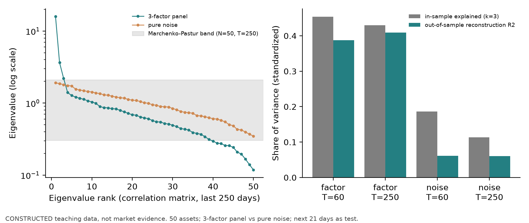
Two constructed return panels have 50 assets and 1,000 days. Factor panel: three factors with daily volatilities of 1.0%, 0.5%, and 0.3%; idiosyncratic volatility of 1.5%; and loadings drawn from $N(0,1)$ (add 1 to the first loading column so average exposure to the market factor is positive). Noise panel: 50 independent columns drawn from $N(0,1.5\%^2)$, with no common factors. Every 21 days, standardize the past $T$ days, fit $k=3$ component PCA, and calculate out-of-sample reconstruction $R^2$ over the next 21 days. Compare that with a single PCA fitted once on all 1,000 days (“full-sample”), also evaluated on each test window.

$^{\mathrm b}$ The three principal-angle cosines between the leading three-dimensional PCA subspaces of adjacent training windows, in descending order, averaged across all adjacent windows.

Interpretation. (1) In the noise panel, the true share for three directions is $3/50=6\%$. Out-of-sample reconstruction is about 6.0%, while in-sample explained variance is 18.6% ($T=60$) and 11.3% ($T=250$), a direct example of the noise bound in Section 6.3. (2) Full-sample PCA gets 8.5% on test windows, higher than the honest 6.0%, because the fit has already seen the test data. The gap is smaller for the factor panel (0.420 versus 0.388) because the factor structure is strong. (3) The final column reports the three principal-angle cosines between adjacent windows' leading three-dimensional PCA subspaces (subspace_cosines): take the singular values of $V_{\text{old}}^\top V_{\text{new}}$ in descending order, then average across adjacent windows. At $T=60$, the smallest average is 0.736, indicating a poorly aligned direction between the two three-dimensional subspaces; the subspace itself changes over time. Principal angles describe the relation between subspaces, not any particular principal-component axis: swapping PC1 and PC3 within the same subspace leaves all three principal-angle cosines at 1, although the corresponding axis cosines are 0, 1, and 0. Thus it is incorrect to say “the third principal component rotated by a certain amount.” The average cosine is also not the average angle because $\arccos$ is nonlinear; $\arccos(0.736)$ is not the average rotation angle. For $T=250$, all three average cosines are approximately 0.988 or higher. The eigenvalues of the final 250-day sample correlation matrix are 15.92, 3.64, and 2.21 for the factor panel; the largest noise-panel eigenvalue is 1.91. The Marchenko–Pastur upper edge is $(1+\sqrt{50/250})^2=2.094$. The factor panel's third eigenvalue is only slightly above the edge, so in real data such a direction can be difficult to distinguish from noise.

8.3 Hand-Calculating One Filtering Step

Two states: daily returns in the calm state (0) follow $N(0.05\%,0.7\%^2)$; in the volatile state (1), they follow $N(-0.1\%,2\%^2)$. Let $P=\begin{pmatrix}0.98&0.02\\0.05&0.95\end{pmatrix}$. Yesterday's closing filtered probability is $\alpha_{t-1}=(0.9,0.1)$, and today's return is $x_t=-2.5\%$.

1. Prediction: $(0.9\times0.98+0.1\times0.05,\ 0.9\times0.02+0.1\times0.95)=(0.887,0.113)$.
2. Densities (units of 1 / decimal return): $\phi(-0.025;0.0005,0.007)=0.0749$ (3.64 standard deviations away), and $\phi(-0.025;-0.001,0.02)=9.709$ (1.2 standard deviations away).
3. Update: $0.887\times0.0749=0.0664$ and $0.113\times9.709=1.0972$. Normalizing gives $\alpha_t=(0.0664,1.0972)/1.1636=(0.057,0.943)$.

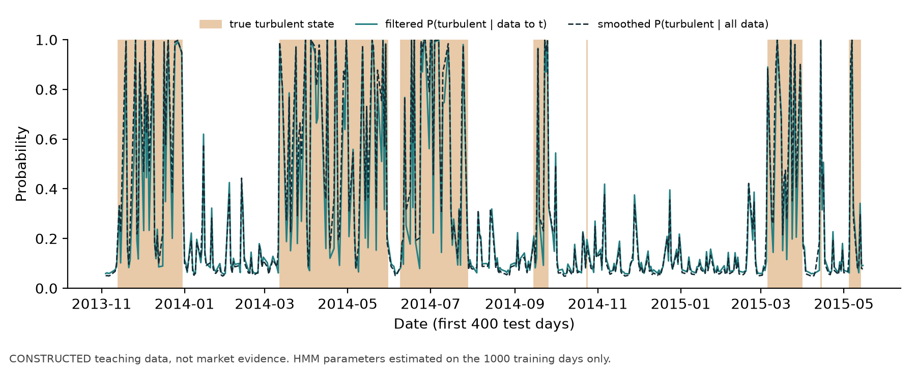
A one-day drop of −2.5% raises the volatile-state probability from 11.3% to 94.3%. If today's return were −1.0%, the two densities would be 18.50 and 18.03, nearly equal, and $\alpha_t=(0.890,0.110)$, so the probability would be determined mostly by the prior. At +0.3%, it would be $(0.955,0.045)$. The script reproduces these three results with hmm_filter_smooth(x=[x_t], init=predicted_probability) (hand.hmm). The stationary distribution is $(5/7,2/7)$, with mean durations of 50 and 20 days.

import numpy as np
from scipy.stats import norm
P = np.array([[0.98, 0.02], [0.05, 0.95]])
pred = np.array([0.9, 0.1]) @ P
for x in (-0.025, -0.010, 0.003):
    lik = np.array([norm.pdf(x, 0.0005, 0.007), norm.pdf(x, -0.001, 0.02)])
    print(x, np.round(pred, 3), np.round(pred * lik / (pred * lik).sum(), 4))

8.4 Regime Timing: Hindsight Labels, Online Labels, and Costs

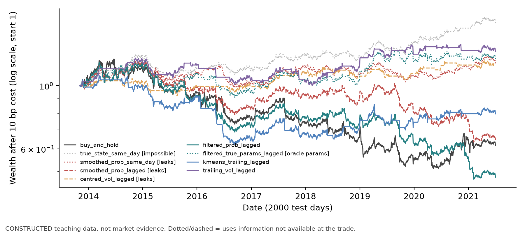
Constructed market: 3,000 days, with states generated from the Markov chain above (seed 4102); the first 1,000 days are the training window and the remaining 2,000 are the test window. The rules use two position sizes: hold the market (weight 1) when classified as calm, and hold cash (weight 0) otherwise. “Lagged” follows the information clock in Section 4: a signal at close $t$ is executed at close $t+1$ (one-day execution lag), then earns the return on day $t+2$. In a daily-return series, this means shifting the signal forward by two periods. “Same-day” aligns the label directly with the return on day $t$ and is only a leakage illustration. A valid rule forms its signal at close $t$, executes at close $t+1$, and earns the return on $t+2$. One-way turnover costs 10 basis points. HMM parameters are estimated on the training window only: a two-component Gaussian mixture provides the means and standard deviations of the states, and a transition matrix is estimated from daily hard-classification counts in the training period with add-one smoothing. This is an approximation using hard classifications from a Gaussian mixture and transition counts; it is not maximum likelihood estimation of the joint HMM likelihood by Baum–Welch. k-means uses past 21-day annualized volatility and 63-day cumulative return, standardized and fitted in the training window with $K=2$. The threshold for the “past volatility” rule is the median volatility in the training window.

Let $u_d$ denote the signal formed at close (distinct from the latent state $s_d$). With returns indexed by their ending date, $r_d=C_d/C_{d-1}-1$. Verify the timing with two adjacent signal dates (the dates below are illustrative trading dates):

The numerical results in this chapter use a fixed-weight-change proxy: $w_d=u_{d-2}$, $\mathrm{turn}_d=|w_d-w_{d-1}|$, and $r_d^{net}=w_dr_d-c\mathrm{turn}_d$. Costs are recorded on the return-ending row. The proxy does not model rebalancing amounts after portfolio-value drift, cash before and after execution, or the event ordering of trades and costs, so it is not equivalent to the event-based self-financing ledger in Chapter 29. The historical proxy numbers and omitted mechanics are retained here; this teaching revision does not silently change the engineering implementation.

Thus, the weight on return-ending date $d$ comes from $u_{d-2}$. Shifting only one period would pair a newly formed signal with a return interval that had already occurred before execution. The “same-day” comparison in the table uses $u_dr_d$ and also violates this clock.

Results from a single path are highly sensitive to chance. As a post hoc robustness diagnostic (D11; not a registered primary result or confirmatory evidence), the same design was repeated with 50 additional seeds. The table shows median Sharpe and the share of paths in which Sharpe exceeded buy and hold on that same path:

There are four takeaways. (1) Same-day hindsight labels earn the most because they use that day's return: after a large daily decline, the smoothed probability classifies that day as volatile, so the rule is “conveniently” out of the market on that day. When the same smoothed probability is executed on the valid schedule ($t+1$ execution, return on $t+2$), median Sharpe falls from 0.76 to 0.05. (2) A centered window uses volatility from the next 10 days, and it still leads when executed on the valid schedule (median 0.63; it beats buy and hold on all 50 paths). “Lagged” does not mean “free of leakage.” (3) Valid online rules retain some value (median 0.29–0.35), well below the leakage-based rules. (4) The HMM estimated on the training window performs worst because of parameter estimation: daily hard classification labels many ordinary calm-period fluctuations as volatile. The estimated transition matrix is $\begin{pmatrix}0.874&0.126\\0.629&0.371\end{pmatrix}$ (true diagonal values 0.98 and 0.95); filtered probabilities switch frequently, generating 38–39 turnovers per year and costs that consume returns. The same filter with true parameters has median Sharpe 0.38. State accuracy and returns do not move together: the training-parameter filter has accuracy 0.856, higher than the past-volatility rule's 0.689, but much lower returns.

Cluster stability on training-window features, using 20 IID row bootstrap samples (a sensitivity check to row perturbations only, not a temporal-stability test): at $K=2$, mean ARI is 0.943 and the minimum is 0.723; at $K=3$, mean ARI is 0.971 and the minimum is 0.815; at $K=4$, mean ARI is 0.722 and the minimum is 0.364. The $K=4$ partition is clearly less stable under resampling. After a true calm-to-volatile transition, the median delay until the filtered probability of calm $P(\text{calm}\mid x_{1:t})$ first falls below 0.5 is 1 day (29 transitions). Figure 2 plots its complement, $P(\text{volatile}\mid x_{1:t})$, and the corresponding first crossing above 0.5. This quick response also comes with many false alarms, which drive turnover.

9. Python Implementation

• Core module: src/quant_course/unsupervised_tools.py.

• Interface contract: Section 2 of qa/a8/ch40_ch41_batch/INTERFACE_CONTRACT.md. Public functions: pca_fit, pca_project, pca_reconstruction_r2, subspace_cosines, trailing_state_features, fit_kmeans_states, assign_states, align_labels, cluster_stability, hmm_filter_smooth, simulate_markov_regimes, and simulate_factor_panel. Tests: tests/test_unsupervised_tools.py.

• Chapter script, approximately 7 seconds. Pass only --out when reproducing results; --figures-dir course/zh/chapters/ch41/figures overwrites the source figures and should be used only when intentionally refreshing them:

  .venv/bin/python code/ch41_unsupervised.py --out <new-output-dir>
  

  Output: results.json and three figures. The command refuses to use an existing output directory.

• Environment: Python 3.14.7, numpy 2.5.3, pandas 3.0.6, scikit-learn 1.9.1, and scipy 1.18.1 (.venv).

• Seeds: factor panel 4101; noise panel 4103; state market 4102; variance-and-predictive-power example 4104; robustness diagnostic 4200–4249. KMeans and Gaussian-mixture random_state values match the corresponding seeds.

• Missing values: pca_fit and pca_project raise an error on NaN (the caller must handle them first); trailing_state_features returns NaN when the window is insufficient; assign_states returns NaN for rows containing NaN, and the rules treat NaN as a flat position.

• Timing: daily frequency; signal at close $t$; execution at close $t+1$; return interval from close $t+1$ to close $t+2$. Leakage-comparison rules are named with [leaks], [impossible], or [oracle params].

Minimal example of training-only PCA and out-of-sample projection:

import numpy as np, pandas as pd
from quant_course import unsupervised_tools as ut
R, B = ut.simulate_factor_panel(300, 20, factor_vols=(0.01, 0.005), idio_vol=0.015, seed=1)
fit = ut.pca_fit(R.iloc[:250], 2, standardize=True)  # mean, SD, loadings: training rows only
scores = ut.pca_project(R.iloc[250:], fit)           # later dates use the training mean/SD
r2 = ut.pca_reconstruction_r2(R.iloc[250:], fit)
print(fit.explained_ratio.round(3), round(r2, 3), scores.shape)

10. Visualization

• Figure 1 (figures/fig41_1_pca_in_vs_out.png, Section 8.2): the horizontal axis is eigenvalue rank and the vertical axis is eigenvalue (log scale); the gray band marks the Marchenko–Pastur range. The right plot's horizontal axis shows four panel/window combinations and its vertical axis shows variance shares. Compare noise eigenvalues with the MP range and in-sample with out-of-sample results.
• Figure 2 (figures/fig41_2_filtered_vs_smoothed.png, Section 8.4): date on the horizontal axis and probability on the vertical axis; observe the “foresight” in smoothed probabilities.
• Figure 3 (figures/fig41_3_regime_rules.png): wealth after 10 basis points of cost across 2,000 test days (log scale, starting at 1). Dashed and dotted lines are rules that use information unavailable at trade time.

11. Real-Market Example

Status: Experiment pending. This course does not have authorization to use a daily stock or index return panel (projects/project06/data_manifest.json; real_data.status = blocked), so this chapter reports no real-market principal components, states, or timing results. To conduct the study, obtain: (1) at least eight years of daily stock returns with point-in-time constituents (including delisted stocks), for training-only PCA, out-of-sample reconstruction $R^2$, and an eigenvalue-bound comparison; (2) daily returns and trading-cost assumptions for a tradable index, for state rules; and (3) permission to display derived statistics in internal training materials. Once the data are available, preregister the windows, $k$, $K$, parameter-estimation method, and costs under the protocol in Section 13.

Literature comparison (not evidence from this book): Laloux et al. (1999) used the return correlation matrix for S&P 500 constituents and found that most eigenvalues fell inside the Marchenko–Pastur range, with only a few (the largest corresponding to the market) clearly outside it. Ang and Timmermann (2012) review applications of regime-switching models in asset pricing. Reading status is documented in Section 20.

12. Common Mistakes

12.1 Full-Sample Standardization and PCA

Mistake: StandardScaler().fit(R) and PCA().fit(R) use all dates, and the resulting scores are treated as daily risk factors or features. Why: test-period means, volatilities, and correlation structure enter the training-period transformation. Impact (noise panel in Section 8.2): full-sample PCA has test-window reconstruction $R^2$ of 8.5%, compared with 6.0% for training-only PCA; the in-sample share is higher at 11.3%–18.6%. Fix: at each rebalance date, fit pca_fit on the past window only and use pca_project on later dates.

import numpy as np, pandas as pd
from quant_course import unsupervised_tools as ut
noise = pd.DataFrame(np.random.default_rng(4103).normal(0, 0.015, (1000, 50)))
noise.columns = [f"A{i:02d}" for i in range(50)]
full = ut.pca_fit(noise, 3, standardize=True)               # WRONG: sees the test window
train = ut.pca_fit(noise.iloc[:250], 3, standardize=True)   # right: training window only
test = noise.iloc[250:271]
print(round(ut.pca_reconstruction_r2(test, full), 3),
      round(ut.pca_reconstruction_r2(test, train), 3),
      round(float(train.explained_ratio.sum()), 3))

The output 0.115 0.077 0.112 means that, on this single 21-day test window, full-sample PCA has reconstruction $R^2$ of 11.5%, training-only PCA has 7.7%, and the training-window in-sample share is 11.2%. Section 8.2 reports averages over all windows (8.5%, 6.0%, and 11.3%).

12.2 Treating Smoothed Probabilities or Hindsight Labels as Trading Signals

Mistake: fit an HMM on the full sample and use smoothed probabilities, or label each day with a “crisis period” confirmed after the fact and align it with the same day's return. Why: the label uses future observations; same-day alignment also uses the return being evaluated. Impact (Section 8.4, median over 50 seeds): the same-day smoothed-probability Sharpe is 0.76, versus 0.05 when executed on the valid schedule (execute at $t+1$, earn the $t+2$ return). Fix: use only filtered probabilities $\Pr(s_t\mid x_{1:t})$, estimate parameters only on the training window, and execute the signal one day later.

12.3 Centered Rolling Windows

Mistake: ret.rolling(21, center=True).std(). Why: the value for date $t$ uses $t+1,\dots,t+10$. Even when the signal is executed at close $t+1$ and earns the return on $t+2$, data from $t+3,\dots,t+10$ still arrive after the return being earned. Impact: median Sharpe over 50 seeds is 0.63, versus 0.35 for the past-window version. Fix: use rolling(21) (right-aligned by default), and test that changing data after $t$ does not change features at $t$ or earlier.

12.4 Unaligned Cluster Labels

Mistake: refit k-means in each window and compare “cluster 1” directly. Why: labels are arbitrary and can switch between fits. Impact: partitions $[0,0,1,1,2,2]$ and $[1,1,0,0,2,2]$ are identical (ARI = 1), but elementwise agreement is only 1/3. Fix: relabel clusters by a meaningful center feature (volatility in this book) or use align_labels for Hungarian matching; ARI itself is label-invariant.

12.5 Selecting Principal Components for Prediction by Explained Variance

Mistake: principal-component regression keeps only components that “explain 99% of the variance.” Why: PCA does not use labels. Impact (constructed example in Section 6.4; first half for training and second half for testing): the first covariance-PCA component explains 98.96% of feature variance, but its out-of-sample $R^2$ is −0.07%; using two components gives 69.6%. After standardization, the first loading is $(0.707,0.707)$ and out-of-sample $R^2$ is 31.2%. Fix: treat $k$ as a hyperparameter and select it by prediction error in date-based training-only validation (as in Project 6 v2's PCA+Ridge ablation in Section 13).

12.6 Evaluating Market Timing by State Accuracy

Mistake: report “85.6% state-classification accuracy” as evidence that a strategy works. Why: accuracy weights each day equally and ignores the size of returns on misclassified days and turnover costs. Impact: the training-parameter filter in Section 8.4 has accuracy 0.856 and Sharpe −0.51; the past-volatility rule has accuracy 0.689 and Sharpe 0.41. Fix: report after-cost returns, turnover, and drawdown together.

13. Quant Research Application

Hypothesis. Do high-variance directions (principal components) of cross-sectional features contain predictive information about future five-day returns? This auxiliary ablation was specified in the Project 6 v2 protocol before v2 runs (configs/p06_trees_v2.json, pca_ridge), not a standalone strategy project. The v1 constructed results had already been viewed; this was not an ex-ante real-market preregistration.

Method. For each outer fold in the date-based walk-forward of Chapter 38, fit StandardScaler, PCA($k$), and Ridge($\alpha$) on training rows only. Select $k\in\{5,15,30\}$ and $\alpha\in\{10^4,10^6\}$ by inner date-validation MSE. Prediction, dollar-neutral portfolios, lagged execution, and cost ledger are otherwise identical to Ridge. Benchmarks are zero prediction, the training mean, and Ridge on the original features.

Controls and interpretation limits. The 43 $q$ and noise series are independent across series and have unit marginal variance, but each follows an AR(1) process with coefficient 0.98. Three additional price features come from the return path and are indirectly related to $q$. The full 46-dimensional feature set is not an IID, homoskedastic population, and finite-sample principal directions are not prespecified signal directions. Truncated PCA may discard signal or reduce estimation variance; which effect dominates must be tested, and improvement cannot automatically be called leakage. A necessary control retains all $k=46$ components, the same training scaler, the same $\alpha$, and no whitening. Under the orthogonal rotation $V$, $\|y-XVb\|^2+\alpha\|b\|^2=\|y-X\beta\|^2+\alpha\|\beta\|^2$, where $\beta=Vb$, so theoretical predictions match original-feature Ridge (apart from numerical error). This equivalence does not hold after truncation, and truncation is not guaranteed to help by denoising. Read historical results by metric and scenario: with the training mean as the $R^2$ benchmark, PCA+Ridge has higher $R^2$ than Ridge in both scenarios, while both remain below zero; its IC is lower in both; its base-case Sharpe at 10/20 bp is lower, while in the sign-reversal case −0.14/−0.52 is slightly higher than Ridge's −0.15/−0.53. Results are in the Project 6 v2 table in Chapter 40, Section 13, and projects/project06/research_report/v2_trees.md.

Clustering and states. This batch does not add cluster states to Project 6: the constructed “sign-reversal” scenario changes the relation between cross-sectional features and returns, while market-level volatility and returns are unchanged. Clustering on market-state features therefore has no identifiable target. A state-rule study requires a separate protocol (Section 17, 41-C02).

14. Chapter Summary

PCA and clustering answer “how are the data distributed?” rather than “what will happen next?” PCA eigenvalues give training-window variance shares. In-sample shares are biased upward by noise; out-of-sample reconstruction $R^2$ and noise bounds provide more honest measures. Scaling determines the directions, and both scaling parameters and components must be estimated within the training window. Clustering depends on scaling, the number of clusters, and initialization; cluster labels have no intrinsic meaning. Row resampling tests sensitivity to row perturbations only; block resampling or rolling refits are needed for temporal stability. State labels divide into three types: online labels and filtered probabilities can be traded; smoothed probabilities and centered windows use future information; hindsight labels aligned with same-day returns also use the return being evaluated. Even valid state rules face parameter-estimation error, detection delay, false alarms, and turnover costs, so evaluate them by after-cost returns rather than classification accuracy.

15. Exercises

41-E01 (by hand) Let $\Sigma=\begin{pmatrix}3&1\\1&3\end{pmatrix}$. Find the eigenvalues, unit loadings (using this book's sign convention), and the first component's explained-variance ratio.

41-E02 (scaling) Two uncorrelated columns have variances 9 and 1. (a) What are the first covariance-PCA loading and explained share? (b) What is special about correlation-matrix PCA after standardization? (c) Using (a) and (b), explain when the “first principal component” depends on the units of measurement.

41-E03 (noise bound) There are $N=100$ independent assets and $T=400$ days. Find the Marchenko–Pastur interval. With no common factors, what share does the first in-sample principal component appear to explain, and what is its true share?

41-E04 (interpretation) Why is a dollar-neutral portfolio with zero market exposure almost unaffected by the first return principal component (which is approximately the market)? What does this say about the relationship between explained variance and portfolio predictive power?

41-E05 (k-means) For one-dimensional data $\{0.10,0.12,0.15,0.30,0.35,0.40\}$, $K=2$, and initial centers 0.10 and 0.15, work through Lloyd iterations to convergence. Show assignments, centers, and objective value (inertia) at every step.

41-E06 (filtering) Use the parameters in Section 8.3. Convert returns, means, and standard deviations to decimal returns for density calculations ($-1\%=-0.010$, $0.7\%=0.007$). Yesterday's filtered probability is $(0.6,0.4)$ and today's return is $-1.0\%$. Find the predicted probabilities, the two densities, and today's filtered probabilities.

41-E07 (timing) Which of the following are available at close $t$ for execution at $t+1$? (a) past 21-day volatility; (b) volatility from rolling(21, center=True); (c) filtered probability with parameters estimated in the training window; (d) filtered probability from an HMM fitted on the full sample; (e) smoothed probability from an HMM fitted on the full sample; (f) nearest-center assignment for past features using k-means fitted in the training window.

41-E08 (cluster labels) What are the ARI and elementwise agreement for partitions $[0,0,1,1,2,2]$ and $[1,1,0,0,2,2]$? What are they for $[0,0,1,1,2,2]$ and $[0,1,0,1,2,2]$?

16. Programming Exercises

41-P01 (training-only PCA) Input: generate 500 days and 30 assets with simulate_factor_panel, factor_vols=(0.01, 0.004), idio_vol=0.015, and seed=7. Implement a rolling window ($T=120$, 20 test days, step size 20) with $k=2$ training-only PCA. Return each window's in-sample explained share and out-of-sample reconstruction $R^2$. Acceptance assertions: (1) for this specified construction and seed, mean in-sample share $\ge$ mean out-of-sample $R^2$; this is not a theorem for arbitrary data or windows; (2) multiplying all data after a given test window by 10 leaves that window and all earlier window results unchanged; (3) the function never re-estimates means or standard deviations on a test window (as a construction check, adding a constant to the entire test window changes out-of-sample $R^2$).

41-P02 (filtering does not look ahead) Use hmm_filter_smooth on the 500-day series from simulate_markov_regimes with p_stay=(0.97, 0.9), mus=(0.0005, -0.001), sigmas=(0.008, 0.02), and seed=3. Acceptance assertions: (1) changing $x_{t+1..T}$ leaves filtered[:t+1] unchanged and changes smoothed[:t+1]; (2) each row sums to 1; (3) verify one update against the numbers in Section 8.3. Boundary condition: at $T=1$, the two probabilities are equal.

41-P03 (state-rule backtest) Given a daily return series and a 0/1 signal, implement the simplified fixed-weight proxy “signal at close $t$, execute at close $t+1$, earn the $t+2$ return, one-way cost $c$” (cost charged on the return-ending row). Return annualized return, Sharpe, turnover, and maximum drawdown (with $N+1$ wealth points). Acceptance assertions: (1) a constant-one signal with $c=0$ matches buy and hold (from day 3 onward); (2) on the Section 8.4 data, the same-day-aligned version using the true state has higher returns than the two-day-lagged version; (3) with $c>0$, at least one nonzero turnover, and positive wealth multipliers at every step, the after-cost terminal wealth is strictly below that for $c=0$; if the portfolio is flat throughout and has zero turnover, they are equal.

17. Challenge Problems

41-C01 (Project 6 v2 PCA ablation) Compare the results and selected $k$ values by fold for pca_ridge in Chapter 40, Section 13, and projects/project06/research_report/v2_trees.md. (a) How do the results compare with the metric-by-metric reference and interpretation limits in Section 13? (b) Give a constructed data-generating process in which PCA+Ridge outperforms Ridge on the original features and explain what real-world situation it represents. (c) Explain why you cannot change the $k$ grid to “exactly the best value” after seeing v2 results and report that result. Additional prerequisite: Chapter 39.

41-C02 (honest state-study design) Design a state-timing study for a tradable index. Specify the number of states, parameter estimation (for example, Baum–Welch EM on training windows only), online signal, execution time, costs, evaluation metrics, benchmarks, out-of-sample period, and falsification condition. Explain how you prevent leakage from Sections 12.2 and 12.3 and how you report the effects of parameter-estimation error (as in the true-parameter comparison in Section 8.4). Additional prerequisites: Chapter 35 on trading costs, Chapter 31 on validation, and Chapter 32 on performance evaluation.

18. Complete Solutions

41-E01. $(3-\lambda)^2-1=0\Rightarrow\lambda=4,2$. For $\lambda=4$, $a=b$, so the loading is $(0.7071,0.7071)$ (positive sum). For $\lambda=2$, $a=-b$, giving a zero sum; choose the first element positive, $(0.7071,-0.7071)$. The explained share is $4/6=66.7\%$.

41-E02. (a) The covariance matrix is $\operatorname{diag}(9,1)$, the first loading is $(1,0)$, and its explained share is 90%. (b) After standardization, the correlation matrix is the identity; both eigenvalues are 1, every unit direction is an eigenvector, and the principal component is not unique. Each direction explains 50%. (c) When columns are weakly correlated and their variance difference mainly reflects their units, the first covariance-PCA component is simply the highest-variance column. Changing that column's units (for example, from percent to decimal) changes the PCA result. For predictive features, standardize using training rows only.

41-E03. $q=100/400=0.25$, so $\lambda_\pm=(1\pm0.5)^2=2.25,\ 0.25$ for a correlation matrix with $\sigma^2=1$. The first in-sample component appears to explain about $2.25/100=2.25\%$; its true share is $1/100=1\%$. This is the upper-edge location under a large-sample limit; the largest finite-sample eigenvalue fluctuates around it.

41-E04. If stock $i$ has return $r_i=\beta_if+e_i$, then a portfolio has return $\sum_iw_ir_i=f\sum_iw_i\beta_i+\sum_iw_ie_i$. When $\sum_iw_i\beta_i=0$, the market term disappears. Dollar neutrality alone does not guarantee this condition. When both dollar neutral and beta-neutral, the portfolio hedges the market direction that explains a large share of common variance; portfolio returns come from other directions (idiosyncratic components or low-variance factors). Thus, the variance share explained by the first component does not by itself determine whether cross-sectional return differences can be predicted.

41-E05. Step 0: with centers 0.10 and 0.15, the midpoint is 0.125. Assign $\{0.10,0.12\}$ and $\{0.15,0.30,0.35,0.40\}$. The objective is $0+0.02^2+0+0.15^2+0.2^2+0.25^2=0.1254$. Updated centers are 0.11 and 0.30. Step 1: the midpoint is 0.205. Assign $\{0.10,0.12,0.15\}$ and $\{0.30,0.35,0.40\}$. The objective (new assignments, old centers) is $0.01^2+0.01^2+0.04^2+0+0.05^2+0.1^2=0.0143$. Updated centers are $0.1233,0.35$. Step 2: the midpoint is 0.2367; assignments are unchanged. The objective is $0.0233^2+0.0033^2+0.0267^2+0.05^2+0+0.05^2=0.006267$. The centers no longer change, so the algorithm converges. The objective decreases monotonically: $0.1254\to0.0143\to0.006267$.

41-E06. Convert the returns, means, and standard deviations to decimal returns first; densities are measured “per unit decimal return,” while normalized state probabilities are dimensionless. The prediction is $(0.6\times0.98+0.4\times0.05,\ 0.6\times0.02+0.4\times0.95)=(0.608,0.392)$. The densities are $\phi(-0.01;0.0005,0.007)=18.50$ and $\phi(-0.01;-0.001,0.02)=18.03$. Normalize $(0.608\times18.50,\ 0.392\times18.03)$ to obtain filtered probability $(0.614,0.386)$. A −1% return is almost equally likely in both states, so the posterior remains close to the prior.

41-E07. Available: (a), (c), and (f). Unavailable: (b), which uses the next 10 days; (d), because although the filtering recursion itself uses only $x_{1:t}$, parameters estimated on the full sample contain test-period information (a subtler form of leakage, usually smaller than (e), but still invalid); and (e), because smoothing uses $x_{t+1:T}$.

41-E08. For the first pair, both partitions group the same points and only swap labels, so ARI = 1; elementwise agreement is $2/6=1/3$. For the second pair, comparing $[0,0,1,1,2,2]$ with $[0,1,0,1,2,2]$, ARI is $1/6\approx0.167$ and elementwise agreement is $4/6$. ARI measures partition agreement and is label-invariant; elementwise agreement depends on the labels and requires alignment first.

41-P01. Reference implementation.

import numpy as np
from quant_course import unsupervised_tools as ut


def rolling_in_out(R, window=120, test=20, k=2):
    rows = []
    for s in range(window, len(R) - test + 1, test):
        fit = ut.pca_fit(R.iloc[s - window:s], k, standardize=True)
        oos = ut.pca_reconstruction_r2(R.iloc[s:s + test], fit)
        rows.append((float(fit.explained_ratio.sum()), oos))
    return np.array(rows)


R, _ = ut.simulate_factor_panel(500, 30, factor_vols=(0.01, 0.004), idio_vol=0.015, seed=7)
a = rolling_in_out(R)
assert a[:, 0].mean() >= a[:, 1].mean()
R2 = R.copy()
R2.iloc[300:] *= 10                 # change only data from row 300 on
b = rolling_in_out(R2)
assert np.allclose(a[:8], b[:8])    # windows whose test ends by row 300 are unchanged
R3 = R.copy()
R3.iloc[120:140] += 0.05
assert not np.isclose(rolling_in_out(R3)[0, 1], a[0, 1])  # shifting the test changes R2
print(a.mean(axis=0).round(3))

The first test window is rows 120–139. The first eight windows end before row 300 and are therefore unaffected. The output reports averages of the two columns. This assertion for a fixed construction does not generalize to all data or establish that out-of-sample performance is always below in-sample performance.

41-P02. Reference implementation.

import numpy as np
from quant_course import unsupervised_tools as ut
m = ut.simulate_markov_regimes(500, p_stay=(0.97, 0.9), mus=(0.0005, -0.001),
                               sigmas=(0.008, 0.02), seed=3)
x = m["ret"].to_numpy()
kw = dict(means=[0.0005, -0.001], sds=[0.008, 0.02],
          transition=np.array([[0.97, 0.03], [0.1, 0.9]]), init=[1.0, 0.0])
f1, s1 = ut.hmm_filter_smooth(x, **kw)
x2 = x.copy()
x2[301:] = -0.05
f2, s2 = ut.hmm_filter_smooth(x2, **kw)
assert np.allclose(f1[:301], f2[:301]) and not np.allclose(s1[:301], s2[:301])
assert np.allclose(f1.sum(axis=1), 1) and np.allclose(s1.sum(axis=1), 1)
P = np.array([[0.98, 0.02], [0.05, 0.95]])
one, _ = ut.hmm_filter_smooth(np.array([-0.025]), means=[0.0005, -0.001], sds=[0.007, 0.02],
                              transition=P, init=np.array([0.9, 0.1]) @ P)
assert np.allclose(one[0], [0.057059, 0.942941], atol=1e-6)
print("ok")

Metric conventions: let $n$ be the number of daily return rows evaluated, including the first two flat days in this exercise. Annualized return is terminal wealth raised to $252/n$ minus 1 (CAGR). Sharpe is $\sqrt{252}$ times the arithmetic mean of daily net simple returns divided by their sample standard deviation (ddof=1); it is not CAGR divided by annualized volatility. Annual turnover is $252\sum\mathrm{turn}/n$. Drawdown includes initial wealth of 1. If the standard deviation is zero, Sharpe is undefined.

41-P03. Reference implementation (same information clock and cost proxy as the book implementation in code/ch41_unsupervised.py; includes all metrics requested by the exercise and checks three assertions. Section 8.4 shifts the full 3,000-day series before taking the test segment; this example slices first and shifts afterward, leaving the first two test days flat, so the numbers differ from Section 8.4):

import numpy as np, pandas as pd
from quant_course import unsupervised_tools as ut


def book(ret, signal, cost, lag=2):
    w = signal.shift(lag).fillna(0.0)
    turn = w.diff().abs().fillna(w.abs())
    net = w * ret - cost * turn
    wealth = np.concatenate([[1.0], np.cumprod(1 + net.to_numpy())])
    n = len(net)
    if n == 0 or np.any(1 + net.to_numpy() <= 0):
        raise ValueError("Require observations and positive wealth multipliers")
    sd = float(net.std(ddof=1)) if n > 1 else float("nan")
    ann_return = float(wealth[-1] ** (252 / n) - 1)
    sharpe = float(np.sqrt(252) * net.mean() / sd) if sd > 0 else float("nan")
    return {"wealth": wealth, "annual_return": ann_return, "sharpe": sharpe,
            "turnover": float(turn.sum()), "annual_turnover": float(turn.sum() * 252 / n),
            "mdd": float((wealth / np.maximum.accumulate(wealth) - 1).min())}


m = ut.simulate_markov_regimes(3000, p_stay=(0.98, 0.95), mus=(0.0005, -0.001),
                               sigmas=(0.007, 0.02), seed=4102)
# The signal is sliced to the test window before shifting, so the first two test days are
# flat; code/ch41_unsupervised.py shifts the full series first (its §8.4 numbers differ).
ret, calm = m["ret"].iloc[1000:], (m["state"].iloc[1000:] == 0).astype(float)
bh = book(ret, pd.Series(1.0, index=ret.index), 0.0)
assert np.isclose(bh["wealth"][-1], np.prod(1 + ret.iloc[2:]))
same_day, lagged = book(ret, calm, 0.001, lag=0), book(ret, calm, 0.001, lag=2)
assert same_day["wealth"][-1] > lagged["wealth"][-1]
assert book(ret, calm, 0.001)["wealth"][-1] < book(ret, calm, 0.0)["wealth"][-1]
print(round(same_day["wealth"][-1], 3), round(lagged["wealth"][-1], 3))

41-C01. Complete reference answer. In the base scenario, PCA+Ridge has $R^2=-0.008\%$ relative to the training mean, versus $-0.113\%$ for Ridge. IC is 0.0135 versus 0.0198, with paired $\Delta IC=-0.0063$ and descriptive $t=-0.86$. Sharpe at 10/20 bp is 0.25/−0.13, below Ridge's 0.45/0.07. In the sign-reversal scenario, $R^2=-0.053\%$ versus $-0.161\%$, IC is 0.0063 versus 0.0087, paired difference is −0.0023, and $t=-0.31$; Sharpe at 10/20 bp is −0.14/−0.52, slightly better than Ridge's −0.15/−0.53. “PCA is worse on every metric” would be inaccurate. Across outer folds 1–16, both scenarios use the same selected-k sequence: [30, 30, 30, 30, 5, 5, 15, 5, 5, 30, 30, 5, 30, 30, 30, 30]. That is 30 components in 10 folds, 5 in 5 folds, and 15 in 1 fold. The frozen summary has no fitdate field, so do not assign dates to these fold numbers. The two scenarios also show that better $R^2$ with respect to the training mean can coexist with lower IC: level error and cross-sectional ranking/portfolio performance are different quantities.

One testable construction makes several features noisy measurements of a common latent variable $z$ and generates labels from $z$ plus label noise. With a finite training sample and a strong common direction associated with $z$, a small number of PCs may aggregate measurement and discard nonpredictive low-variance directions, potentially outperforming Ridge on the original features; this is not guaranteed. Retain the full-$k$ orthogonal-equivalence control, use the same scaler and $\alpha$, and do not whiten; compare using training-only validation. This represents a setting where many correlated indicators measure the same economic quantity, not a mechanism already validated by this project.

Changing the $k$ grid to its best value after viewing test results turns the outer test set into a selection set. A new idea can be tested in a new version, with the prior results disclosed, the original grid and negative results retained, and independent later dates used for evaluation; the old test data cannot be relabeled as unseen. PCA is a compression tool, and these constructed results do not support a market-alpha claim.

41-C02. Complete protocol example. First confirm the index, total-return series, tradable instrument, and data permission; fix the training period and unseen test dates. Use only past 21-day volatility and 63-day return as state features, with the scaler estimated within each training window. Fix $K=2$, or compare 2 and 3 using training-only date validation and select by likelihood and stability, not test returns. Fit the HMM with Baum–Welch EM from multiple initializations within each training window; record initial values, convergence, likelihood, and transition matrices. Do not describe Gaussian-mixture hard-classification transition counts as maximum likelihood for the joint HMM. Freeze parameters, filter forward, form the signal at close $t$, execute at close $t+1$, and earn the return ending at $t+2$. Check that perturbing future data does not change earlier features or filtered probabilities.

For the actual strategy, use the Chapter 29 event ledger, one-way costs of 0/10/20 bp, and explicit assumptions for impact and financing. If a teaching proxy is also shown, state separately that it charges costs on the return-ending row and explain how it differs from the event ledger. Use buy and hold and a past-volatility rule as benchmarks. Report annualized return, Sharpe, drawdown, and turnover; results in crisis and calm periods; and results across initializations and rolling windows. Full-sample smoothing and centered windows are unavailable-to-trade diagnostics only and cannot be selected into the strategy. Interpret state labels from training-window centers; ARI does not require label alignment, while temporal stability requires block perturbation or rolling refits.

Before looking at test results, specify a decision rule; for example, do not adopt the strategy if its after-cost performance is no better than the past-volatility rule, its advantage appears in only one subperiod, or it is highly sensitive to initialization. A simulation with true parameters can serve as an unavailable oracle reference, not a guaranteed upper bound on after-cost returns or Sharpe: compare estimated and true transition matrices, false alarms and delay, turnover, and cost loss. Section 8.4's true-parameter median Sharpe of 0.38 versus −0.03 with training-estimated parameters shows that estimation error deserves investigation, but does not guarantee that EM will move estimates toward the true values. Real markets have no known true states or parameters; do not treat this simulation difference as a market result. Without authorization, real-market work remains blocked.

19. Further Reading

• Must know: Jolliffe and Cadima (2016), Section 2: choosing between covariance and correlation-matrix PCA and interpreting explained variance. Relevant to Sections 5–6.
• Should know: Laloux, Cizeau, Bouchaud, and Potters (1999): using random-matrix bounds for financial correlation matrices and assessing whether sample eigenvalues exceed noise. Hamilton (1989), Sections 3–4: Markov-switching models and filtered/smoothed probabilities.
• Advanced: Ang and Timmermann (2012): a review of regime switching in asset pricing; read Sections 2 and 4. Connor and Korajczyk (1986): statistical factor models based on asymptotic principal components. von Luxburg (2010): theory and limitations of clustering stability.
• Optional: scikit-learn 1.9.1 documentation for PCA, KMeans, and adjusted_rand_score, to check implementation details.

20. References

Reading statuses below refer to the original course author’s historical review recorded in source_notes; BIL19 inherits those statuses without reopening publications or performing new online verification.

Full links and reading locations are in references.md, references/sources.json, and this chapter's source_notes.md.

• NUMPY: NumPy documentation (linalg.eigh). Used for eigendecomposition in Sections 6.1 and 8.1. Reading status: based on the local 2.5.3 implementation.
• SK_PITFALLS: scikit-learn “Common pitfalls” (data leakage and training-only preprocessing). Used for scaling in Section 5 and Section 12.1. Reading status: carried forward from A8-A.
• CH41_JC2016: Jolliffe, I. T., & Cadima, J. (2016). Principal component analysis: a review and recent developments. Phil. Trans. R. Soc. A, 374, 20150202. Used in Section 5 and Section 6.2 on scaling. Reading status: the AMC reconnaissance report covered Section 2(c); the author did not reread it.
• CH41_LCBP1999: Laloux, L., Cizeau, P., Bouchaud, J.-P., & Potters, M. (1999). Noise dressing of financial correlation matrices. Physical Review Letters, 83, 1467–1470. Used for the bound and assumptions in Section 6.3 and for Section 11. Reading status: see source_notes.md.
• CH41_HAMILTON1989: Hamilton, J. D. (1989). A new approach to the economic analysis of nonstationary time series and the business cycle. Econometrica, 57(2), 357–384. Used for the HMM in Section 5 and filtering and smoothing in Section 6.6. Reading status: the reconnaissance report (R); the author did not read the full text.
• CH41_AT2012: Ang, A., & Timmermann, A. (2012). Regime changes and financial markets. Annual Review of Financial Economics, 4, 313–337. Used in Section 11 and Section 19. Reading status: reconnaissance report (R); the author did not read the full text.
• CH41_CK1986: Connor, G., & Korajczyk, R. A. (1986). Performance measurement with the arbitrage pricing theory. Journal of Financial Economics, 15(3), 373–394. Used in Section 19. Reading status: abstract only.
• CH41_VL2010: von Luxburg, U. (2010). Clustering stability: an overview. Foundations and Trends in Machine Learning, 2(3), 235–274. Used for cluster stability in Section 5 and Section 19. Reading status: reconnaissance report (R); the author did not read the full text.
• SK_KMEANS_DOC: scikit-learn 1.9.1 KMeans and adjusted_rand_score (documentation in local source). Used for k-means and ARI in Section 5. Reading status: checked by the author against local source documentation.

Specific passages read, reader, and which sources were consulted only at abstract level are recorded in course/zh/chapters/ch41/source_notes.md.

Notebook Reader Entry

The I3 Chapter 41 notebook has 12 cells, including 6 code cells. It freshly calculates the hand example, four PCA combinations, variance versus prediction, a 3,000-day state path, and the D11 post hoc diagnostic over seeds 4200–4249; it writes two new figures to a new RUN_DIR. It is not a frozen replay. This diagnostic is not promoted to a preregistered primary result. The notebook's bilingual projection is handled by BIL23; this batch did not run or modify the notebook.