Quality

Through line: Quality is not a single number. It has several accounting dimensions: profitability, leverage, the cash content of earnings, and stability. For each dimension, ask what the numerator is, what the denominator is, whether both come from the same financial-statement version, and whether the market knew them at that point in time. Prerequisites: Chapter 12 (financial statements), Chapter 23 (cross-sectional research), and Chapter 24 (value and point-in-time fundamentals). After this chapter, you should be able to decompose ROE into net margin, turnover, and the equity multiplier, and explain why rising ROE does not necessarily mean better operations; distinguish ending from average denominators and handle negative or near-zero equity; calculate gross profit to assets, operating profitability to equity, accrual ratios, and earnings stability; construct ratios from one financial-statement version; explain financial-sector conventions; and interpret the published RMW factor return while recognizing that it does not test an individual-stock quality signal.

1. Chapter goals

Readers should be able to answer: Is a company “high quality” because it truly earns more, or because it borrows more? Does a number in an earnings ratio represent cash, and was it public at the time?

1. State the numerator, denominator, unit, direction, and relevant industries for ROE, ROA, GP/A, OP, leverage, the accrual ratio, and earnings stability.
2. Use the DuPont decomposition $\mathrm{ROE}=\text{net margin}\times\text{asset turnover}\times\text{equity multiplier}$ to derive the effect of leverage, $\mathrm{ROE}=\rho+(\rho-i)D/E$, and use two companies to show how “operating improvement” and “more leverage” can produce similar ROE changes.
3. Explain the choice between average and ending balances, why negative or near-zero equity makes ROE meaningless, and why both year-end equity balances must be positive before averaging them.
4. Apply the “same financial-statement version” rule: numerator and denominator must come from the same filing; a restated numerator cannot be divided by a pre-restatement denominator.
5. Reproduce with a constructed panel that net-income measures mix in accruals; most cross-sectional ROE variance comes from leverage; near-zero equity can severely distort Pearson IC; Spearman is more robust to extreme magnitudes, but ranks and sample filtering can still change it; and the Pearson composite identity for two uncorrelated standardized dimensions, then compare it in scale with a constructed rank IC.
6. Read published monthly RMW returns and report the mean, $t$-statistic, subperiods, drawdown, and correlations; explain that this describes an aggregate factor return and does not test any stock-level quality signal.

Completion criterion: Every quality signal includes a field table specifying each field’s reporting period, available_at, ingested_at, unit, and industries where it is undefined.

2. Why Quant needs this

A value factor asks, “Is the price cheap relative to fundamentals?” A quality factor asks, “Are the fundamentals themselves good?” Together, they provide more information available in advance for identifying value traps: a company that is cheap but unprofitable, highly leveraged, or supported by accruals may rank well on value and poorly on quality. Chapter 28 combines the two, but every quality metric must stand on its own before combination.

Quality metrics have the same difficulty as value metrics, but it is less visible. The numerator comes from the income statement (a flow over a period), while the denominator comes from the balance sheet (a stock at a point in time); their time conventions naturally differ. The denominator is often equity close to zero or even negative. Profit and liabilities mean different things in financial firms. Net income includes amounts unsupported by cash. Financial statements may be restated. Chapter 24’s point-in-time selection rules apply directly, with one additional rule: the numerator and denominator of a ratio must come from the same version.

The chapter proceeds as follows: define the measures (Section 5); derive why leverage changes ROE (6.1); address denominators (6.2), measures that do not directly contain a financing multiplier (6.3), accruals (6.4), estimation error in stability (6.5), same-version selection (6.6), and financial firms (6.7); quantify how standardized dimensions combine (6.8); and finish with a constructed panel and published RMW returns (Sections 10–11).

3. Intuition

Last year, two companies both raised ROE from 15% to 20%. Company A cut costs and sold more effectively, so it earned more profit per dollar of sales. Company B borrowed money to repurchase shares, shrinking its equity; the same profit divided by less equity raised ROE. Both ROEs rose, but A improved its operations while B took on more risk. Decomposing ROE into “margin × turnover × leverage” reveals the difference.

Another common confusion is profit versus cash. Net income is an accounting number. Part of it comes from changes in receivables, inventory, and accrued expenses and does not correspond to cash received. If the profit-cash difference comes from accruals that later reverse, it may be followed by lower earnings. Investment, seasonal working capital, and accounting classifications can also cause a difference; its direction must be tested. Subtracting net cash from operating activities from net income, then dividing by average assets, gives the accrual ratio. It measures the gap between accounting earnings and operating cash flow; it is not “cash” itself.

A third issue is timing. A financial statement may be released weeks after the fiscal year ends, and its reported values may later be revised. For every number in a quality signal, ask: who could see it at the signal month-end?

Simplifying boundary: the constructed panel in this chapter represents these phenomena with a minimal structure (one latent quality factor, one accrual tendency, and random leverage). Real-company accounting is much more complex.

3.1 One available filing, worked through completely

4. Mathematical foundations

Notation. For company $i$ and a fiscal year, let sales be $S$, cost of goods sold be $C$, selling, general, and administrative expenses be $G$, interest expense be $I$, net income attributable to common shareholders be $N$, operating cash flow be $F$, total assets be $A$, debt be $D$, and book equity be $E=A-D$. Note that this is a simplification for this chapter: it assumes all liabilities are interest-bearing debt $D$. A real balance sheet also has non-interest-bearing operating liabilities such as accounts payable and deferred revenue; equity is $A-L$, where $L\ge D$ is total liabilities. Both the DuPont derivation and the constructed panel use $E=A-D$; with real statements, distinguish interest-bearing debt from total liabilities. Income-statement items are flows over a fiscal year; balance-sheet items are stocks at fiscal year-end. Use one currency and scale. Flow-to-balance ratios must carry an annual window (in continuous-time units, per year, including asset turnover, ROE, and GP/A). In this course, fixed fiscal-year cumulative flows divided by balances are shown as unitless decimals or percentages, while debt/assets and the equity multiplier are stock-to-stock ratios. Neither convention describes monthly investment returns.

Average balances. Profit earned during a fiscal year corresponds to average assets during that year. A common calculation is $\bar A=(A_{\text{year-end}}+A_{\text{year-start}})/2$; use the same convention for $\bar E$. The year-start balance is the prior fiscal year-end balance. A 10-K reports balance sheets for both the current and prior years, so both balances can come from one filing.

DuPont identity. When $S,A,E>0$,

The three factors are net margin, asset turnover, and the equity multiplier (also called financial leverage).

Precision of the sample standard deviation. For $n$ independent normal observations, the variance of sample standard deviation $s$ is approximately $\sigma^2/(2(n-1))$, with relative standard error $1/\sqrt{2(n-1)}$.

Combining two signals. Let standardized signals $z_1,z_2$ be uncorrelated with variance 1, and a standardized label $y$ have variance 1 and correlations $\rho_1,\rho_2$ with the two signals. Then $\mathrm{Corr}(z_1+z_2,\,y)=\dfrac{\rho_1+\rho_2}{\sqrt2}$.

Frequency convention: accounting quantities are annual; signals and returns are monthly. signal_time is month-end, and the signal uses the most recent fiscal year that was available.

5. Formal definitions

Return on Equity (ROE). $N/\bar E$, using average or ending common equity as the denominator; undefined when equity is nonpositive.

Return on Assets (ROA). $N/\bar A$. It does not use equity, but net income has already deducted interest, so ROA contains some leverage information.

Gross Profitability (GP/A). $(S-C)/\bar A$. Gross profit is revenue minus cost of goods sold. Novy-Marx’s 2012 author manuscript records gross profits-to-assets, normalized by book assets rather than equity. The course and P4 use average assets as the course-interface convention; do not attribute “average” to a paper definition that has not been checked. The numerator does not directly deduct interest. Financial firms have no cost-of-goods-sold field in this sense, so this measure does not apply to them.

Operating Profitability (OP). Fama and French’s (2015, note to Table 8) definition is $(S-C-G-I)/E$: revenue minus cost of goods sold, SG&A, and interest expense, divided by book equity. Include only firms with positive book equity. The numerator deducts interest and the denominator is equity, so OP contains leverage.

Leverage. This chapter uses both $D/A$ (debt to total assets, unitless; between 0 and 1 in the simplified model with $E=A-D>0$, but it can exceed 1 for a real company with nonpositive equity) and the equity multiplier $A/E$. These describe capital structure, not profitability.

Accrual ratio. $(N-F)/\bar A$: net income minus net cash from operating activities, divided by assets. It measures the size of the difference between net income and operating cash flow relative to average assets: the higher the value, the larger the portion by which net income exceeds operating cash flow (scaled by assets); the lower or more negative the value, the more operating cash flow exceeds net income. It is not “the proportion of profit not yet received in cash.” Company A has $N=10$, $F=5$, and $\bar A=100$, so $a=5\%$ and the difference is 50% of net income. Company B has $N=20$, $F=12$, and $\bar A=100$, so $a=8\%$, while the difference is only 40% of net income. To discuss the difference as a share of net income, define a separate ratio $(N-F)/N$ and handle $N\le0$ separately.

Earnings stability. The sample standard deviation of the most recent $n$ fiscal years of ROA (or ROE); lower means more stable. Usually $n=5$; fewer than $n$ years gives NaN.

Same-version rule. The numerator and denominator used to form a ratio must come from the same financial statement and version. After a restatement is released, recalculate using all values from the restated filing; before it is released, continue to use the original values.

RMW (Robust Minus Weak). A published profitability-factor spread: $\tfrac12(\text{Small Robust}+\text{Big Robust})-\tfrac12(\text{Small Weak}+\text{Big Weak})$, formed from six value-weighted portfolios sorted on size and operating profitability (French database description page). It is an aggregate return, not a stock-level signal.

Convention for using “quality.” In this chapter, “quality” refers only to the calculable accounting dimensions above, not unmeasured concepts such as management or a moat. Different studies combine dimensions differently; this chapter does not call any one combination “the standard definition of a quality factor.”

6. Derivations

6.1 DuPont decomposition and the effect of leverage on ROE

Consider a company with debt $D$ and an after-tax borrowing cost $i$. Compare cases with fixed assets, operating return, and debt interest; require positive equity and assume all liabilities are this debt. After-tax quantities must be matched under the simplifying conditions of a common tax rate, deductible interest, and a tax shield usable in the current period. Do not assume an immediate tax shield unconditionally when the company has severe losses. Let net operating profit after tax (NOPAT) be $=\rho A$, where $\rho$ is the after-tax return on operating assets. Net income is NOPAT minus after-tax interest: $N=\rho A-iD$. Equity is $E=A-D$. Therefore,

The identity used is $A/E=1+D/E$. Interpretation: with no debt ($D/E=0$), ROE equals $\rho$. If $\rho>i$, every additional unit of $D/E$ raises ROE by $(\rho-i)$. For $\rho=8\%, i=3\%$, values $D/E=0,0.5,1,2$ give ROE of $8\%,10.5\%,13\%,18\%$. Thus ROE can rise solely because leverage rose, while $\rho$ stays unchanged. DuPont splits the change into three factors: leverage changes the third factor, $A/E$; operating improvement changes the first and second. Section 8.1 works through two companies numerically.

The cost of leverage: the same $D/E$ lowers ROE when $\rho<i$ and increases ROE volatility (the multiplier amplifies variation in $\rho$). A company whose high ROE comes from high leverage is more fragile.

6.2 Denominators: average, ending, and near-zero equity

Sensitivity of ROE to the denominator. $\mathrm{ROE}=N/E$, $\partial\mathrm{ROE}/\partial E=-N/E^2$, and a first-order approximation gives relative change $\delta\mathrm{ROE}/\mathrm{ROE}\approx-\delta E/E$. With equity $E=400$, a one-unit equity error changes ROE by about 0.25% in relative terms (not 0.25 percentage points). With equity $E=2$, a one-unit error is so large that the first-order approximation fails: increasing equity from 2 to 3 lowers ROE by 33%; decreasing it from 2 to 1 raises ROE by 100%. With $N=40$, equity of 2 gives $40/2=2000\%$; equity of 3 gives $40/3=1333.3\%$, a drop of 666.7 percentage points; equity of 1 gives $40/1=4000\%$, a rise of 2000 percentage points. Near-zero equity turns accounting noise into extreme values.

Negative equity. When $E<0$ and $N>0$, $N/E$ is negative; when $E=0$, the ratio is undefined. Both are excluded under the course rule. The negative-equity ratio looks like “very poor profitability” but actually reflects insolvency; the sign has changed meaning. This chapter requires positive equity, consistent with Fama–French’s inclusion condition (French database description page).

Average-balance trap. Ending equity is $-30$ and beginning equity is 100. The simple average is 35, which is positive, and $N=40$ gives ROE $=114\%$: a very high profitability figure for a company insolvent at year-end. Therefore, require both balances to be positive before averaging them (average_balance(..., floor=0.0)).

Near-zero equity. Even positive equity may need a floor; for example, require equity to exceed 5% of assets (the floor parameter). The threshold is a research choice: write it into the plan and report the fraction excluded.

Ending versus average balances. Profit is a flow accumulated over the fiscal year, so average balances match it better. Ending balances refer to fiscal year-end and are simpler to use; that reference date does not mean they have been publicly released or locally ingested. Both ending and average conventions must wait until the same filing satisfies the available_at/ingested_at cutoff. The two are similar for companies with stable growth, but can differ substantially when equity changes rapidly (Section 8.3: $N=40$, equity falls from 500 to 100; ending ROE is 40%, average ROE is 13.3%). State the denominator choice in the plan and use a consistent convention across metrics.

6.3 Why gross profit to assets does not directly contain a financing multiplier

Net income $N=(S-C-G-I-\cdots)(1-\tau)$ includes interest $I$, which equals debt times the interest rate, so $N$ is related to capital structure. Gross profit $S-C$ is before interest. Dividing it by assets $A$ (the total capital, regardless of whether it is debt or equity) neither subtracts interest nor uses a denominator tied to the financing structure. Therefore, in a comparison with sales, costs, and assets held fixed, borrowing interest or an equity denominator does not directly change GP/A; it measures gross profit per asset. Actual borrowing can affect investment, working capital, and operating costs, so this does not imply statistical independence between real-world GP/A and leverage. OP deducts interest in the numerator and uses equity in the denominator, so it is affected by leverage. That is the substantive difference between the measures, not an implementation detail.

6.4 Accruals: the gap between earnings and cash

Net cash from operating activities $F$ is operating cash flow on the cash-flow statement; net income $N$ is measured on an accrual basis. The difference $N-F$ is the total accrual gap. It includes working-capital changes, depreciation, and other noncash items, and is also affected by cash-flow-statement classification. Working-capital changes (receivables, inventory, accounts payable, and so on) and noncash items such as depreciation can contribute. The accrual ratio is $a=(N-F)/\bar A$. A high $a$ means net income exceeds operating cash flow by more relative to assets; $F$ is itself a net cash amount, so $N-F$ does not identify, transaction by transaction, which profit has not yet been received in cash. If accruals later reverse, future earnings may fall. This is a mechanism hypothesis; the direction and size of accruals’ predictive relation with returns is an empirical question (this chapter has not read Sloan 1996 and does not restate its results). Direction convention: lower raw accrual ratio $a$ is better; the quality signal is $-a$, so higher transformed values are better. Do not mix up the direction of the raw ratio and its negative.

6.5 Estimation error in earnings stability

Measure stability with the sample standard deviation $s_n$ of ROA over $n$ years. Suppose annual ROA is approximately independent and normal, with population standard deviation $\sigma_i$. Then $\mathrm{Var}(s_n)\approx\sigma_i^2/(2(n-1))$, with relative standard error $1/\sqrt{2(n-1)}$: 35% for $n=5$ and 24% for $n=10$. Thus, when ranking companies by five-year standard deviation, two companies whose true volatilities differ by 30% can easily be ranked in the opposite order in the sample. These values show that a short-history standard deviation has low relative precision; they do not prove it is noisier than every level estimate, whose precision also depends on the mean, volatility, sample size, and dependence structure. Practical implication: assign NaN when a company has fewer than $n$ years; do not fill a five-year measure with a two-year standard deviation. When combining stability with level metrics, lower its weight or use a longer window. This is an approximation under normality and independence. Financial data often have serial dependence and heavy tails, so estimate actual error according to the data’s dependence structure; this approximation cannot establish that stability is always noisier.

6.6 Same-version rule: a false change caused by a restatement

Suppose a company originally reports $N=40$, $E=400$, and ROE $=10\%$. It later restates the values to $N=28$, $E=350$. Using one version gives $40/400=10\%$ before the restatement and $28/350=8\%$ afterward. If only the numerator is updated after the restatement while the denominator remains from the original version (combining the database’s “latest net income” with the “first ingested equity”), the result is $28/400=7\%$: an apparent change of $-3$ percentage points, versus the true $-2$ percentage-point change, overstated by 1 percentage point. Worse, using the restated values before the restatement was released is look-ahead (Chapter 24, Section 6.4). Therefore, retrieve an entire row at once with latest_available_values; all numerators and denominators must come from that row. This includes the prior year-end balance (the comparative balance in the same 10-K), which is why assets_prev and equity_prev are stored in the same row.

6.7 Financial firms

Banks and insurers have balance sheets dominated by financial liabilities. Interest is both a cost and operating revenue, and they do not have cost of goods sold in the same sense; the numerators for GP/A and OP are undefined, as are EV and EBITDA (Chapter 24). A bank’s equity multiplier is often around 10, versus 1 to 2 for a nonfinancial company, so the same ROE has a different meaning in the two industries. Treatment: set GP/A and OP to NaN for financial firms (Novy-Marx’s author manuscript also excludes them); rank ROE and ROA within industry; report coverage for each metric. In the constructed panel, the median bank equity multiplier is about 11.2, versus about 1.5 for nonfinancial companies.

6.8 Combining two standardized dimensions: the arithmetic of correlation

The following is an identity for standardized Pearson variables on the same paired sample. Uncorrelated does not mean independent; the specified correlation matrix must be valid, and the composite variance must be nonzero. Let $z_1,z_2$ be standardized and uncorrelated, and $y$ standardized, with $\mathrm{Corr}(z_k,y)=\rho_k$. Then $\mathrm{Cov}(z_1+z_2,y)=\rho_1+\rho_2$, $\mathrm{Var}(z_1+z_2)=2$, and the correlation of the composite signal is $(\rho_1+\rho_2)/\sqrt2$. In the constructed panel, IC is 0.0241 for GP/A and 0.0418 for $-$accruals; latent quality and accrual tendency are independent by construction, and the average same-date rank correlation of the two signals is $-0.073$ (near zero, but not zero). Under zero correlation, the prediction is $(0.0241+0.0418)/\sqrt2=0.0466$. Adjusting for $r_{12}=-0.073$ gives $0.0659/\sqrt{2(1+r_{12})}=0.0659/1.362=0.0484$. The measured IC of the equal-weighted rank average is 0.0473, between the two predictions. This is a scale comparison only: averages across dates of Rank IC and rank correlation do not exactly obey the single-sample standardized Pearson identity. Conditions: the two signals are uncorrelated, weights are equal after separately standardizing each signal, and weights are not tuned on the test period. If their correlation is $r_{12}>0$, the denominator becomes $\sqrt{2(1+r_{12})}$ and the composite gain shrinks. This is the starting point for Chapter 28’s discussion of factor correlations and weighting.

7. Financial interpretation

Quality has multiple dimensions. Profitability levels (GP/A, OP, ROA, ROE) ask “how much does the company earn?” Leverage asks “how much does it rely on borrowing?” Accruals ask “how much cash is in earnings?” Stability asks “how volatile are earnings?” Dimensions can point in opposite directions: a highly leveraged company can have high ROE but be fragile; a company with high accruals can report high earnings but little operating cash. Before compressing them into one “quality score,” know what each dimension measures.

ROE mixes in leverage. In the constructed panel, cross-sectional variance of ROE is 5.6 times that of ROA (0.0233 versus 0.0042). The mean leverage $D/A$ of the top ROE quintile, averaged across dates, is 0.419; for the bottom quintile it is 0.342; and for the full sample it is 0.340. The high-ROE group is more leveraged. Leverage in the top and bottom GP/A quintiles is nearly identical (0.332 and 0.329). These are numerical illustrations of the mechanisms in Sections 6.1 and 6.3.

Net-income measures contain accruals. In the constructed panel, profit $N$ includes an accrual component negatively related to returns (a construction assumption). Net-income measures ROA (IC 0.0113) and ROE (0.016) are therefore weaker than GP/A, which does not contain accruals (0.0241). This does not show that GP/A is better in real markets. It shows only that if net income mixes in a component related to future returns in the opposite direction, using net income directly dilutes the signal. Whether real-world accruals have this direction must be tested with data.

The relation between quality and value is an empirical question. Fama and French (2015, Section 7) find that value stocks tend to have weaker profitability unconditionally; after controlling for other factors, value stocks behave like robustly profitable stocks. In the constructed panel, quality and value are independent by design, so it cannot answer this question. Published RMW and HML returns have correlation 0.095 (Section 11).

Economic meaning of RMW. Published RMW averages 0.25% per month ($t=3.03$) over 1963–2026. It is an aggregate spread before costs and financing. It does not show which accounting metric is better or whether an individual-stock portfolio bought on quality can be implemented.

Availability timing. As in Chapter 24, Novy-Marx’s author manuscript starts using a fiscal year’s accounting data at the end of June in the next calendar year; Fama–French’s RMW also forms in July of year $t$ using fiscal-year $t-1$ data. Researchers must state their own lag rule.

7.1 Why profitability might relate to next-period returns

High profitability does not automatically imply high stock returns: if the price already fully reflects those cash flows, a buyer gets no free excess return. A risk hypothesis might ask whether highly profitable companies have lower risk and therefore lower required returns, or how different quality dimensions behave in bad states. A mispricing hypothesis might ask whether investors underweight earnings persistence or underreact to differences between cash and accruals. A proxy hypothesis might ask whether a measure stands in for industry, size, asset measurement, or leverage. Each question requires observations and tests designed in advance; the word “quality” alone does not imply a positive premium.

The accrual gap especially requires economic judgment. A growing company may increase receivables, temporarily making operating cash flow lower than profit; it may also be recognizing revenue aggressively. The same accrual ratio does not identify the cause. The course’s constructed panel builds a negative effect of accrual tendency on returns into its generator to demonstrate how the signal behaves under that assumption; it does not decide the mechanism for real companies. The original Sloan and Piotroski papers have not been read here, so no empirical results from them are added. RMW is a published portfolio spread and cannot substitute for single-stock GP/A or OP fields; it also does not test the accounting quality in this example.

8. Numerical worked examples: calculate each step

All numbers are generated by hand_examples() and independently checked using a different implementation in qa/a5/claude/recompute/ch26_recompute.py. The companies are constructed for teaching.

8.1 Same increase in ROE: operating improvement versus more leverage

This section uses a simplified DuPont calculation with ending balances, unlike P4’s average balances in Section 3.1. Amounts are in millions of dollars. Last year, Companies A and B were identical: net income 60, sales 1000, total assets 600, and equity 400. ROE $=60/400=15\%$; net margin $60/1000=6\%$; turnover $1000/600=1.667$; equity multiplier $600/400=1.5$; product $0.06\times1.667\times1.5=15\%$.

This year, Company A’s net income rises to 90 and everything else stays fixed: margin 9%, turnover 1.667, multiplier 1.5, and ROE $=22.5\%$—an operating improvement. Company B borrows 100 to repurchase shares: equity falls to 300, debt rises by 100, after-tax interest is about 3.75, and net income is $60-3.75=56.25$. Sales and assets do not change. Margin falls to $5.625\%$, turnover remains 1.667, the multiplier is $600/300=2.0$, and ROE is $0.05625\times1.667\times2=18.75\%$. Company B’s margin falls even as ROE rises; the increase comes from the multiplier.

8.2 Effect of leverage on ROE

Let $\rho=8\%$ and after-tax debt cost $i=3\%$. For $D/E=0,0.5,1,2$, ROE is $8\%,10.5\%,13\%,18\%$ (using $\mathrm{ROE}=\rho+(\rho-i)D/E$). Balance-sheet check: assets 200, debt 100, equity 100, NOPAT $=0.08\times200=16$, after-tax interest $0.03\times100=3$, net income 13, and ROE $=13/100=13\%$.

8.3 Denominator: ending, average, and near-zero equity

Let $N=40$ and assets be 1000.

Interpretation: ending and average values differ most for companies whose equity changes rapidly. Averaging can hide negative ending equity by turning it positive (and reporting ROE of 114%). With a threshold, near-zero equity becomes NaN; report the fraction excluded.

8.4 Gross profit, operating profitability, and accruals

A company in this simplified example has identical beginning and ending assets, so 800 is also same-version average assets; the accrual example likewise uses 500 as average assets. Sales are 1000, cost of goods sold 600, SG&A 200, interest 20, total assets 800, and book equity 400. GP/A $=(1000-600)/800=50\%$; OP $=(1000-600-200-20)/400=45\%$. If interest is 60, GP/A is unchanged and OP is $=(1000-600-200-60)/400=35\%$: OP falls with leverage while GP/A does not. Two companies have net income 50 and assets 500. Company A’s operating cash flow is 80, so its accrual ratio is $(50-80)/500=-6\%$ (operating cash exceeds net income by 30). Company B’s operating cash flow is 20, so the ratio is $+6\%$ (net income exceeds operating cash by 30, or 6% of assets).

8.5 False change from mixing versions

Originally, $N=40,E=400$ (ROE 10%); after restatement, $N=28,E=350$. Same-version ROE after restatement is $28/350=8\%$; the mixed-version result is $28/400=7\%$. The change from 10% to 7% is -3 percentage points, while the true same-version change from 10% to 8% is -2 percentage points.

8.6 Estimation error in stability

For a five-year standard deviation of ROA, relative standard error is $1/\sqrt{2\times4}=0.354$. Suppose two companies’ true standard deviations are 4% and 5.2%, a 30% difference. Each sample standard deviation has 35% relative error, so the sample ranking can readily reverse. Under a normal approximation, the standard deviation of the log ratio of two independent estimates is about $\sqrt{2}\times0.354=0.5$; the true log ratio $\ln1.3=0.26$ is only half a standard deviation, implying about a 30% chance of reversal. The exact value from the $F$ distribution is 31%.

8.7 Combining two dimensions

Let $\rho_1=0.0241$ and $\rho_2=0.0418$. Then $(\rho_1+\rho_2)/\sqrt2=0.0466$. If the signals have correlation 0.5, $\sqrt{2(1+0.5)}=1.732$, and composite correlation is $0.0659/1.732=0.0380$, 18% lower than when they are uncorrelated.

9. Python implementation

Field definitions are in the new module quality.py. Same-version fundamental selection reuses Chapter 24’s latest_available_values, which can retrieve multiple columns at once with the entire row from one version. Ranking and IC reuse Chapter 23’s factor_research.py.

Default offline entry point (run from the I3 reader-package root):

.venv/bin/python run_notebook.py notebooks/ch26_quality.ipynb

The default is RUN_FRENCH=False. The stability example uses 100,000 worlds and seed 11 (the body’s historical example uses 200,000). The composite example uses 400,000 observations and resets seed 5 for each $r_{12}$ (the body uses 600,000 and a continuous RNG). quality_world and quality_study default to seed 20261107. The runner also writes an execution copy and status under runs/execution_<stem>_<uuid>/. The notebook’s English-language layer and package-wide paths are assembled in BIL23. The following historical full CLI and test references are not the default offline command:

.venv/bin/python code/ch26_quality.py
.venv/bin/python -m pytest tests/test_ch26_quality.py tests/test_ch26_workflow.py -q

By default, this builds only a chapter-level RUN_DIR and does not write CSV, PNG, or JSON files or generate a historical figure library.

Frequency: accounting measures are annual; signals and returns are monthly. signal_time is the final instant of month-end (UTC). Version selection follows Chapter 24, Section 6.4, using latest_available_values. Each filing contains both the current and prior-year balance sheets, so average balances come from the same filing. CLI seed: 20261107.

Code segment one: DuPont decomposition and leverage effect (Sections 8.1 and 8.2).

import pandas as pd

from quant_course.quality import dupont, roe_from_leverage

idx = pd.period_range("2026-06", periods=1, freq="M")
mk = lambda v: pd.DataFrame([[v]], index=idx, columns=["f"])
before = dupont(mk(60.0), mk(1000.0), mk(600.0), mk(400.0))
ops = dupont(mk(90.0), mk(1000.0), mk(600.0), mk(400.0))          # operations improve: margin 6% -> 9%
lev = dupont(mk(56.25), mk(1000.0), mk(600.0), mk(300.0))         # buy back 100 of equity with debt; after-tax interest 3.75
r = lambda d, k: float(d[k].iloc[0, 0])
assert abs(r(before, "roe") - 0.15) < 1e-12 and abs(r(ops, "roe") - 0.225) < 1e-12 and abs(r(lev, "roe") - 0.1875) < 1e-12
assert r(lev, "net_margin") < r(before, "net_margin") and r(lev, "equity_multiplier") > r(before, "equity_multiplier")   # ROE rose although margin fell
assert abs(roe_from_leverage(0.08, 0.03, 1.0) - 0.13) < 1e-12 and abs((16 - 0.03 * 100) / 100 - 0.13) < 1e-12              # balance-sheet check
print(round(r(ops, "roe"), 4), round(r(lev, "roe"), 4))

Code segment two: denominator rules (Section 8.3).

import numpy as np
import pandas as pd

from quant_course.quality import average_balance, guarded_ratio

idx = pd.period_range("2026-06", periods=1, freq="M")
cols = ["steady", "shrinking", "tiny", "negative"]
ni = pd.DataFrame([[40.0] * 4], index=idx, columns=cols)
end = pd.DataFrame([[400.0, 100.0, 2.0, -30.0]], index=idx, columns=cols)
prev = pd.DataFrame([[400.0, 500.0, 300.0, 100.0]], index=idx, columns=cols)
assets = pd.DataFrame([[1000.0] * 4], index=idx, columns=cols)
roe_end = guarded_ratio(ni, end).iloc[0]
roe_avg_unguarded = guarded_ratio(ni, average_balance(end, prev)).iloc[0]
roe_avg = guarded_ratio(ni, average_balance(end, prev, floor=0.0)).iloc[0]
roe_floor = guarded_ratio(ni, end, floor=0.02 * assets).iloc[0]
assert abs(roe_end["tiny"] - 20.0) < 1e-12 and np.isnan(roe_end["negative"])                       # 2000%, and no ratio for negative equity
assert abs(roe_avg_unguarded["negative"] - 40 / 35) < 1e-12                                          # the average hides the negative balance: 114%
assert np.isnan(roe_avg["negative"]) and abs(roe_avg["shrinking"] - 40 / 300) < 1e-12
assert np.isnan(roe_floor["tiny"]) and abs(roe_floor["shrinking"] - 0.4) < 1e-12                    # 2 < 2% of assets (20): dropped
print(pd.DataFrame({"ending": roe_end, "average, unguarded": roe_avg_unguarded, "average, both > 0": roe_avg, "ending, 2% floor": roe_floor}).round(3))

Code segment three: GP/A, OP, accruals, and leverage (Section 8.4).

import pandas as pd

from quant_course.quality import accrual_ratio, gross_profit_to_assets, operating_profitability

idx = pd.period_range("2026-06", periods=1, freq="M")
mk = lambda *v: pd.DataFrame([list(v)], index=idx, columns=["low_debt", "high_debt"][: len(v)])
rev, cogs, sga = mk(1000.0, 1000.0), mk(600.0, 600.0), mk(200.0, 200.0)
interest, assets, equity = mk(20.0, 60.0), mk(800.0, 800.0), mk(400.0, 400.0)
gpa = gross_profit_to_assets(rev, cogs, assets).iloc[0]
op = operating_profitability(rev, cogs, sga, interest, equity).iloc[0]
assert (gpa == 0.5).all()                                                                       # GP/A ignores interest
assert abs(op["low_debt"] - 0.45) < 1e-12 and abs(op["high_debt"] - 0.35) < 1e-12              # OP falls when interest rises
acc = accrual_ratio(mk(50.0, 50.0), mk(80.0, 20.0), mk(500.0, 500.0)).iloc[0]
assert abs(acc["low_debt"] + 0.06) < 1e-12 and abs(acc["high_debt"] - 0.06) < 1e-12            # cash-backed vs not (columns reused as labels)
print(gpa.to_dict(), op.round(3).to_dict(), acc.round(3).to_dict())

Code segment four: same-version rule and restatement (Section 8.5).

import pandas as pd

from quant_course.factor_signals import latest_available_values
from quant_course.quality import guarded_ratio

versions = pd.DataFrame({
    "security_id": ["S1", "S1"], "period_end": pd.to_datetime(["2022-12-31", "2022-12-31"]),
    "available_at": pd.to_datetime(["2023-03-15 16:05", "2023-11-20 16:05"], utc=True),
    "ingested_at": pd.to_datetime(["2023-03-15 16:12", "2023-11-20 16:12"], utc=True),
    "net_income": [40.0, 28.0], "equity": [400.0, 350.0]})                              # restated NI and equity
months = pd.period_range("2023-10", "2023-11", freq="M")
pit = latest_available_values(versions, months, ["net_income", "equity"])
same_version = guarded_ratio(pit["net_income"], pit["equity"])["S1"]
old_equity = latest_available_values(versions, months[:1], ["equity"])["equity"]["S1"].iloc[0]   # the equity known in October, kept after the restatement
mixed_nov = pit["net_income"]["S1"].iloc[1] / old_equity
assert abs(same_version.iloc[0] - 0.10) < 1e-12 and abs(same_version.iloc[1] - 0.08) < 1e-12
assert abs(mixed_nov - 0.07) < 1e-12                                                      # new numerator over the old denominator: a false -3 pp change
print(same_version.round(3).to_dict(), round(mixed_nov, 3))

Code segment five: estimation error in earnings stability and probability of a rank reversal (Sections 6.5 and 8.6).

import numpy as np

rng = np.random.default_rng(11)
worlds = 200_000
from scipy import stats

for n in (5, 10):
    expected = float(stats.f.sf((0.06 / 0.04) ** 2, n - 1, n - 1))            # exact: s1^2/s2^2 = (sigma1/sigma2)^2 F(n-1, n-1); 0.226 and 0.121
    s1 = rng.normal(0.0, 0.04, (worlds, n)).std(axis=1, ddof=1)             # true sigma 4%
    s2 = rng.normal(0.0, 0.06, (worlds, n)).std(axis=1, ddof=1)             # true sigma 6% (50% higher)
    reversed_share = float((s1 > s2).mean())                                  # sample ranking opposite to the truth
    assert abs(reversed_share - expected) < 0.01                              # the lognormal approximation (0.209, 0.112) is a little low
    print(n, round(reversed_share, 3), round(1 / np.sqrt(2 * (n - 1)), 3))

Code segment six: IC after combining two uncorrelated signals (Sections 6.8 and 8.7).

import numpy as np

rng = np.random.default_rng(5)
rho1, rho2, n = 0.0241, 0.0418, 600_000


def composite_ic(r12: float) -> float:
    """Correlation of z1 + z2 with y when corr(z1, y) = rho1, corr(z2, y) = rho2 and corr(z1, z2) = r12."""
    cov = np.array([[1.0, r12, rho1], [r12, 1.0, rho2], [rho1, rho2, 1.0]])
    z1, z2, y = rng.multivariate_normal(np.zeros(3), cov, size=n).T
    return float(np.corrcoef(z1 + z2, y)[0, 1])


zero, half = composite_ic(0.0), composite_ic(0.5)
assert abs(zero - (rho1 + rho2) / np.sqrt(2)) < 0.004 and abs(half - (rho1 + rho2) / np.sqrt(2 * 1.5)) < 0.004
assert half < zero                                                              # a correlated second signal shrinks the gain
print(round(zero, 4), round(half, 4))

10. Reading the figures

Figure 26-1: Leverage, ROE, and near-zero equity. Left: with an after-tax debt cost of 3% (dashed line), three curves show ROE against $D/E$ for operating returns $\rho=4\%,8\%,12\%$. When $\rho>i$, ROE rises with slope $\rho-i$; when $\rho<i$, it falls. Right: ROE for 300 nonfinancial companies in one month of the constructed panel. The left column uses unguarded ending-equity ROE; the right uses average equity with both balances positive and requires equity to exceed 5% of assets. The unguarded column has extreme values (hundreds of percent); the guarded values fall into a more reasonable range. Interpretation: near-zero-equity outliers are not economic information. Constructed data.

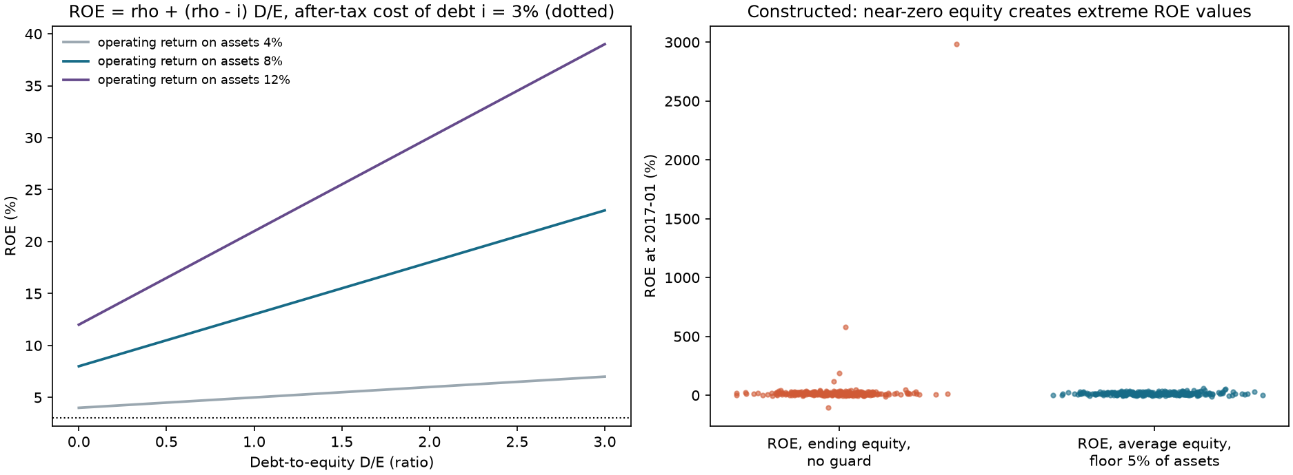
Figure 26-2: IC for different quality measures. Constructed panel with 300 nonfinancial companies and 132 months, using fixed seed 20261107. Bars show mean Spearman IC (vertical lines are approximately plus or minus two standard errors), in order: ROE (ending equity), ROE (average equity), ROE (average equity with equity above 5% of assets), ROA, GP/A, OP, $-$accruals, $-$leverage, and the equal-weighted rank average of GP/A and $-$accruals. Interpretation: net-income measures (ROE, ROA) are weaker than gross profit (GP/A) and operating profitability (OP); $-$accruals is strongest, and the composite is strongest; $-$leverage is near zero (leverage is unrelated to returns by construction). These are results of the constructed setup, not estimates for real markets.

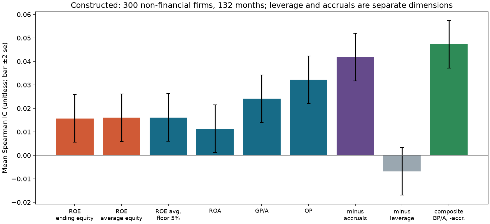
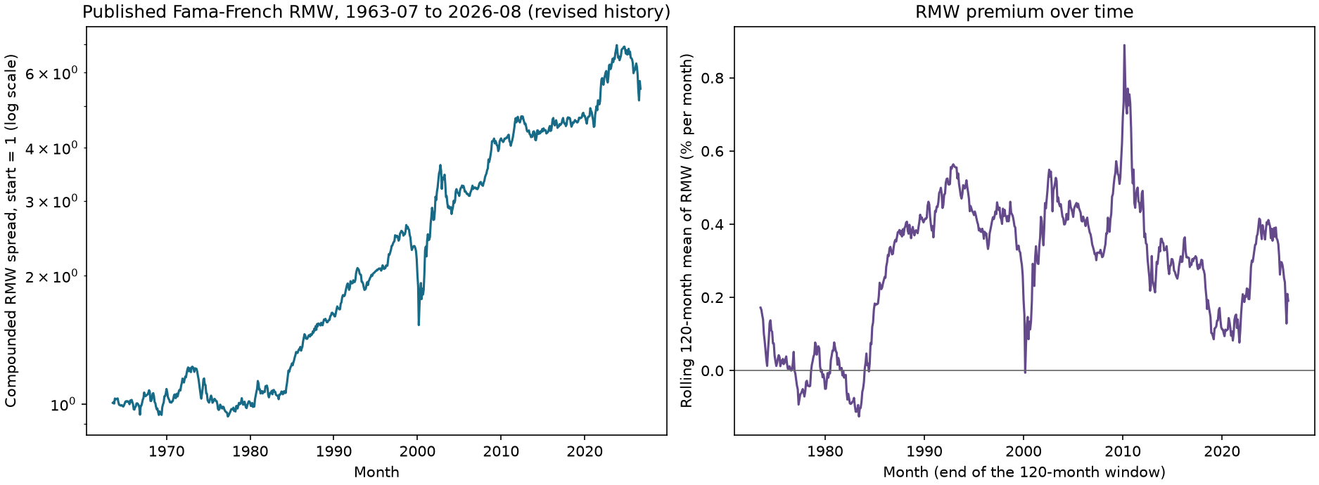
Figure 26-3: Published RMW. Left: compounded cumulative RMW monthly spread (log scale, starting at 1, July 1963 through August 2026). Right: rolling 120-month mean RMW (percent per month). Interpretation: a slow long-run rise, positive most of the time, with a drawdown around 2000 (maximum drawdown about 42%, occurring in 2000-02). This is a published aggregate spread, before costs and financing.

11. Historical market case

Data and limitations. Use the French five-factor (2×3) monthly data frozen on 2026-10-05: Ken French Data Library: F-F Research Data 5 Factors 2x3. The processed CSV has SHA-256 833bd925b49651428781c789c13a6ac7454d4676449e6d119782050046a57eea and 758 months (July 1963 through August 2026), in decimal monthly spread returns. Publicly downloadable does not mean freely redistributable. RMW construction is described in Section 5 and the source notes: six value-weighted portfolios are formed by size and operating profitability using fiscal year $t-1$, formed in July and held through the following June; only firms with positive equity and available revenue and cost items are included. This is a published aggregate return, not a stock-level profitability signal, not point-in-time statement-version data, and not an execution record.

Descriptive results.

Maximum drawdown of compound returns is 41.8%, occurring in 2000-02. Correlation with market excess return is $-0.19$, with SMB $-0.33$, with HML $+0.10$, and with CMA $+0.02$. The reported $t$-statistics treat months as independent observations and are naive; the two subperiods were selected after the fact, so their $t$-statistics are not confirmatory tests. Volatility is notably higher after 2000 (2.98% versus 1.60%).

What can and cannot be said. We can say that the published profitability spread averaged positive returns over 1963–2026; mean returns are positive in both subperiods, while standard deviations differ by nearly a factor of two; RMW is negatively correlated with SMB and nearly uncorrelated with HML. We cannot say: (1) that any one accounting metric (GP/A, OP, ROE, or accruals) is the better quality measure, since RMW uses only operating profitability; (2) that high-OP individual stocks earn higher returns, since RMW is the arithmetic difference of six value-weighted portfolios; (3) what the quality–value relation is for individual stocks: Fama–French’s (2015, Section 7) unconditional and conditional descriptions apply to their sample, and this chapter has no individual-stock test; or (4) that the strategy is tradable, has capacity, or is profitable after costs.

What is missing for stock-level quality research. We need every version and available_at for each company-year’s revenue, cost of goods sold, SG&A, interest, net income, operating cash flow, assets, equity, and debt; historical stock universes and delistings; historical industry classifications; prices and market capitalizations. The SEC Financial Statement Data Sets listed in Chapter 24 provide as-filed XBRL values and acceptance timestamps from 2009 onward, but mappings from tags (Extensible Business Reporting Language, XBRL, labels) to accounting concepts and coverage/consistency of items such as cost of goods sold require separate review; the datasets do not contain prices or delisting returns. No such data were downloaded for this chapter. The Project 4 preparation-layer gap table lists these items.

12. Common mistakes

Mistake 1: interpreting higher ROE as operating improvement. Section 8.1: Company B’s margin falls while its ROE rises. Fix: always report the three DuPont factors, or use GP/A, which does not directly deduct interest, in a comparison holding operations and assets fixed; report leverage as well. ROA uses net income after interest and still contains financing information.

Mistake 2: averaging away negative equity. Section 8.3: ending equity $-30$ and beginning equity 100 average to 35, producing ROE of 114%. Fix: require both balances to be positive before averaging.

Mistake 3: allowing near-zero equity into the ranking. In the constructed panel, Pearson IC for unguarded ending-equity ROE is 0.0017 ($t=0.36$), rising to 0.0177 ($t=3.22$) after the guard. Spearman ICs in this construction are similar (0.0157 and 0.0161). Spearman is robust to extreme magnitude changes that do not alter ranks, but changes in ranks, pairwise reordering after filtering, and changes in the universe can still affect it. Fix: set a denominator threshold and report exclusions; use Rank IC by default for rank-based signals.

import numpy as np
import pandas as pd

from quant_course.factor_research import information_coefficient
from quant_course.quality import guarded_ratio

rng = np.random.default_rng(8)
n = 300
quality = rng.standard_normal(n)
equity = np.exp(rng.normal(5.0, 0.3, n)); equity[:6] = [1.0, 0.5, 2.0, 0.8, 1.5, 3.0]          # six near-zero equity firms
income = 40 + 15 * quality + rng.normal(0, 5, n)
ret = 0.01 * quality + 0.03 * rng.standard_normal(n)
idx = pd.period_range("2026-06", periods=1, freq="M")
frame = lambda v: pd.DataFrame([v], index=idx, columns=range(n))
raw = guarded_ratio(frame(income), frame(equity)).iloc[0].to_numpy()                            # no floor: ROE of ~4000% for the tiny firms
guard = guarded_ratio(frame(income), frame(equity), floor=frame(np.full(n, 20.0))).iloc[0].to_numpy()
p_raw, p_guard = information_coefficient(raw, ret, method="pearson"), information_coefficient(guard, ret, method="pearson")
s_raw = information_coefficient(raw, ret, method="spearman")
assert p_guard > p_raw + 0.1 and abs(s_raw - information_coefficient(guard, ret, method="spearman")) < 0.1
print(round(p_raw, 3), round(p_guard, 3), round(s_raw, 3))

Mistake 4: mixing versions. Section 8.5: using a new numerator over an old denominator gives a 3-percentage-point decline instead of the true 2-point decline, an extra 1-point drop. Fix: select the whole row at once.

Mistake 5: calculating GP/A or OP for financial firms. Banks have no cost of goods sold in this definition; replacing revenue with interest income and cost with interest expense produces a different measure. Fix: set these two metrics to NaN for financial firms, rank ROE and ROA within industry, and report coverage. In the constructed panel, all bank GP/A values are NaN (CLI assertion).

Mistake 6: treating net income as cash. Section 8.4: two companies with the same net income have operating cash flow of 80 and 20; this does not identify, transaction by transaction, which profit was received in cash. Fix: calculate the accrual ratio separately and read net-income measures alongside accruals.

Mistake 7: ranking stability from only a few years. Sections 6.5 and 8.6: the relative error of a five-year standard deviation is 35%; the probability that sample ranks reverse for two companies whose true standard deviations differ by 30% is about 30%. When the true difference is 50% (26-E06), the exact reversal probabilities are about 23% for 5 years and 12% for 10 years. Fix: require enough years, reduce the weight, or use a longer window.

Mistake 8: tuning composite weights on the test period. The composite assumptions in Sections 8.7 and 6.8 set equal weights in advance. Choosing weights based on test-period IC inflates the composite IC through post hoc selection (Chapter 22). Fix: fix weights in the plan or estimate them only in the training period.

13. Quantitative research application

Quality field contract (Project 4 signal layer).

Research workflow (constructed panel). Freeze a plan: the hypothesis that companies with higher gross profit to assets and a lower accrual ratio on the same date have higher next-month returns; the signal is the equal-weighted average of the same-date percentiles of those two dimensions; the primary statistic is the $t$-statistic of Rank IC. Evaluate each dimension first, then the composite; fix weights before observing returns. Results: 132 months and 300 nonfinancial companies; GP/A Rank IC 0.0241 ($t=4.58$), $-$accruals 0.0418 ($t=8.31$), composite 0.0473 ($t=9.00$, hit rate 72.5%); mean monthly returns for the highest and lowest GP/A quintiles are 1.039% and 0.594%, a long-short spread of 0.445% ($t=4.26$). These directions and magnitudes are known under the constructed setup, so they demonstrate that the functions and workflow behave as specified, not a real-world effect.

Constraints for Project 4. (1) Retrieve an entire row at once with latest_available_values for every ratio. (2) Report coverage and exclusions for each metric. (3) Handle financial firms separately. (4) Report net-income measures together with accruals and leverage. (5) Require enough years for stability. (6) Fix composite weights in advance; multiple dimensions enter Chapter 28’s factor-correlation and crowding analysis. (7) Record every variant in Chapter 22’s ledger.

13.1 Metric mapping and coverage: first ask “who is still rankable?”

The current P4 quality fields are only gp_a, neg_accrual, and roe_avg, with formulas corresponding to 44.4444%, +3.3333%, and 25.7143% in Section 3.1. The current seven fields do not include OP. The standalone quality.operating_profitability function is available for teaching; the existence of this function does not mean P4 has integrated OP. The paper’s gross profits-to-assets, the course’s average-asset GP/A, and French’s equity-denominator OP are three distinct definitions; do not substitute one for another. RMW is a portfolio return formed under French’s convention, not company-level OP input.

P4’s actual roe_avg guard operates in two steps: average_balance(equity, equity_prev, floor=0.0) first excludes any record with a nonpositive year-end equity balance; then guarded_ratio(..., floor=0.05 * assets_avg) excludes average equity that is not strictly greater than 5% of average assets. A value equal to the threshold is excluded. This is a prespecified interface threshold, not a universal definition of ROE. The 2% threshold in Section 8.3 and the 5% ending-equity threshold in 26-E03 are separate teaching-policy examples and must not be described as the P4 rule.

Consider four companies with average assets of 1000 and net income of 40, and beginning/ending equity as follows: A (80,120), B (10,30), C (120,-20), and D (40,60). Company A has average equity 100, greater than 50, so ROE of 40% is valid. B has average equity 20, at or below 50, and is excluded. C is excluded first because ending equity is nonpositive (its unguarded average is exactly 50). D’s average equity is 50, equal to the threshold, and is excluded. Of four companies with complete inputs, only one passes: valid ROE coverage is 25%, with 75% lost. Accruals or GP/A may still be available according to their own fields. Missingness is not a zero quality score. Report coverage by size and industry and each failure reason, since filtering may systematically change the universe.

Raw quality fields enter the unified winsorization, industry/size residualization, standardization, and synthesis flow in Chapter 24, Section 13.1. Missing GP/A for financial firms changes which dimensions are available; renormalizing within style does not restore missing economic evidence. A residualized quality score and the final weight projection by industry are separate stages. Distinguish older A6 weights outside the support from C13’s limited correction: listed-support projection, gross restoration to 2, and the 60-name threshold are accepted; execution and drift residuals are reported separately. See the current-interface entry in Chapter 24, Section 13.1. Real eligibility, borrowing, fees, capacity, and a complete real-data P4 remain unfinished; old outputs have not thereby been rerun.

14. Chapter summary

Quality comprises several accounting dimensions. ROE is the product of net margin, turnover, and leverage; leverage can raise ROE without improving operations: $\mathrm{ROE}=\rho+(\rho-i)D/E$. GP/A does not directly deduct interest and does not directly contain an equity-financing multiplier when operations and assets are held fixed. Net-income measures mix in accruals. The accrual ratio is the net-income/operating-cash-flow gap scaled by average assets, not the gap as a share of earnings. A five-year earnings-standard-deviation estimate has about 35% relative error and noisy rankings. Denominators must be positive and away from zero; require both year-end balances to be positive before averaging; draw the numerator and denominator from the same financial-statement version; handle industries without cost of goods sold separately. For two uncorrelated dimensions, composite IC is approximately $(\rho_1+\rho_2)/\sqrt2$; correlation reduces the gain. Published RMW averages 0.25% per month ($t=3.03$), is an aggregate spread, and does not test stock-level signals. Scope: effects in the constructed panel are assumptions; RMW is revised historical data; this chapter has no point-in-time stock-level data.

15. Exercises

26-E01 (by hand). A company’s first-year net income is 36, sales 600, total assets 400, and equity 150. In year two, net income is 39.6, sales 660, total assets 440, and equity 110 (it borrowed to repurchase shares). Calculate net margin, turnover, equity multiplier, and ROE for both years; explain the source of the ROE change.

26-E02 (by hand). Operating return $\rho=10\%$, after-tax debt cost $i=4\%$, and $D/E=1.5$. Find ROE. Then set $\rho=3\%$ and $i=4\%$; find ROE and interpret its sign.

26-E03 (by hand). Net income is 24 and assets are 800. Three companies have (beginning equity, ending equity): (200, 180), (150, 6), and (80, $-10$). Find ending ROE, unguarded average ROE, average ROE only when both balances are positive, and ending ROE subject to ending equity being above 5% of assets.

26-E04 (by hand). Revenue is 2400, cost of goods sold 1500, SG&A 500, interest 100, total assets 2000 (same-version beginning and ending assets are both 2000, so average assets are also 2000), and book equity is 800. Find GP/A and OP. If interest is 300, what are the two values? With net income 120, operating cash flow 60, and average assets 1000, what is the accrual ratio? What if operating cash flow is 180?

26-E05 (by hand). Originally, net income is 55 and equity is 500; after restatement, net income is 44 and equity is 440. Find both same-version ROEs, the value using the new numerator over the old denominator, and the false change caused by mixing versions.

26-E06 (calculation). What is the relative standard error of a standard deviation estimated over 5 years and over 10 years? If two companies’ true standard deviations are 4% and 6%, what are the approximate probabilities that their sample rankings reverse using 5-year and 10-year samples?

26-E07 (calculation). Two standardized signals have correlations $\rho_1=0.03$ and $\rho_2=0.02$ with the label. What is the IC of the equally weighted composite if they are uncorrelated and if their correlation is 0.3?

26-E08 (concept and calculation). A bank has ROA of 1% and an equity multiplier of 11; a software company has ROA of 8% and an equity multiplier of 1.5. Calculate both ROEs and explain why ranking them by ROE across the full market is inappropriate. What alternative would you use?

26-N01 (filing version and coverage). Recalculate the five ratios in Section 3.1 and label the sign, denominator, and annual unit; explain why February values are unavailable and why French OP does not switch to average equity. Use the four companies in Section 13.1 to check P4’s ROE threshold and coverage loss, and explain why GP/A and RMW cannot be substituted for each other.

16. Programming exercises

26-P01. Use dupont to reproduce 26-E01 and assert that the entire ROE change comes from the equity multiplier (net margin and turnover are unchanged). Acceptance criterion: assertions for all three factors pass.

26-P02. Construct a version table with one restatement, use latest_available_values to retrieve numerator and denominator together, and assert the ROEs before and after restatement as well as that “new numerator over old denominator” differs from both. Acceptance criterion: all three assertions pass.

26-P03. Simulate two signals with correlation 0.5 and correlations 0.03 and 0.02 with the label. Calculate the IC of their equally weighted composite and compare it with $({\rho_1+\rho_2})/{\sqrt{2(1+r_{12})}}$. Acceptance criterion: error below 0.005.

17. Challenge problems

26-C01 (derivation). Extend Section 6.1. Let pretax operating profit (earnings before interest and taxes, EBIT) over assets be $r_a=\mathrm{EBIT}/A$, tax rate be $\tau$, and pretax debt rate be $r_d$. Derive $\mathrm{ROE}=(1-\tau)\bigl[r_a+(r_a-r_d)D/E\bigr]$ and explain the mapping to $\rho$ and $i$ in Section 6.1. Discuss the effect of leverage on ROE and ROE volatility when $\rho<i$. Prerequisite: identity $A/E=1+D/E$. Grading: derivation 50, mapping 20, discussion 30.

26-C02 (open-ended). For a Project 4 quality signal, write a data-gap table and frozen plan. For every field, state whether it exists in the course’s current data, a source where real data could be obtained, its time fields, and missing-data rules. Explain which conclusions cannot be written without these data. List the three checks required before combining quality and value: correlation, coverage, and timing. Grading: gap table 30, frozen plan 30, claims that cannot be made 20, pre-combination checks 20.

18. Complete solutions and reference implementations

26-E01. Year one: net margin $36/600=6\%$, turnover $600/400=1.5$, equity multiplier $400/150=2.667$, and ROE $=36/150=24\%$ (the product $0.06\times1.5\times2.667=0.24$). Year two: net margin $39.6/660=6\%$, turnover $660/440=1.5$, equity multiplier $440/110=4.0$, and ROE $=39.6/110=36\%$. Margin and turnover do not change; the multiplier rises from 2.667 to 4.0, accounting for all 12 percentage points of ROE increase.

26-E02. $\mathrm{ROE}=0.10+(0.10-0.04)\times1.5=0.19$. When $\rho=3\%<i=4\%$, $0.03+(0.03-0.04)\times1.5=0.015$ (1.5%). Leverage lowers ROE below $\rho$ because asset returns are below borrowing costs; more borrowing loses more.

26-E03. Ending ROEs: $24/180=13.3\%$; $24/6=400\%$; and $24/(-10)=-240\%$ (the sign has lost its meaning, so report NaN). Unguarded averages: $(200+180)/2=190\to12.6\%$; $(150+6)/2=78\to30.8\%$; and $(80-10)/2=35\to68.6\%$. Require both balances positive before averaging: 12.6%, 30.8%, NaN. Require ending equity greater than 5% of assets (40): 13.3%, NaN ($6<40$), NaN ($-10<40$). The third company’s 68.6% is an artifact of averaging away insolvency at year-end.

26-E04. GP/A $=(2400-1500)/2000=45\%$; OP $=(2400-1500-500-100)/800=37.5\%$. With interest of 300, GP/A remains 45%; OP is $=(2400-1500-500-300)/800=12.5\%$. Accrual ratios: $(120-60)/1000=+6\%$ and $(120-180)/1000=-6\%$.

26-E05. Same version: original $55/500=11\%$ and restated $44/440=10\%$, a true change of $-1$ percentage point. Mixing gives $44/500=8.8\%$, an apparent change of $8.8-11=-2.2$ percentage points, 1.2 percentage points more decline than the true change.

26-E06. Relative standard error $1/\sqrt{2(n-1)}$: 0.354 for $n=5$ and 0.236 for $n=10$. The standard deviation of the log ratio of two independent estimates is approximately $\sqrt2$ times the relative standard error: 0.5 for $n=5$ and 0.333 for $n=10$. The true log ratio is $\ln(6/4)=0.405$. Under the normal approximation for the log ratio, reversal probabilities are $\Phi(-0.405/0.5)=\Phi(-0.81)=0.209$ for $n=5$ and $\Phi(-0.405/0.333)=\Phi(-1.216)=0.112$ for $n=10$. These are approximations and slightly low. The exact sample-variance ratio satisfies $s_1^2/s_2^2\sim(\sigma_1/\sigma_2)^2F(n-1,n-1)$, giving $P(F_{n-1,n-1}>2.25)=0.226$ for $n=5$ and 0.121 for $n=10$. The simulation in Section 9, code segment five, centers around the exact values.

26-E07. If uncorrelated: $(0.03+0.02)/\sqrt2=0.0354$. If correlation is 0.3: $0.05/\sqrt{2(1+0.3)}=0.05/1.612=0.0310$.

26-E08. Bank ROE $=1\%\times11=11\%$; software ROE $=8\%\times1.5=12\%$. Their ROEs are close, but net income/assets (ROA) differs by a factor of eight. ROA here already deducts interest, so it is not the operating return $\rho$ before financing in Section 6.1. The bank’s 11% comes with 11-fold leverage; the software company’s 12% comes from asset profitability. Ranking by ROE across the whole market puts very different risks on one scale. Rank within industry and interpret alongside financing and asset definitions; for nonfinancial companies GP/A may also be examined. Handle financial firms separately; do not describe ROA as excluding leverage.

26-P01 reference implementation

import pandas as pd

from quant_course.quality import dupont

idx = pd.period_range("2026-06", periods=1, freq="M")
mk = lambda v: pd.DataFrame([[v]], index=idx, columns=["f"])
y1 = dupont(mk(36.0), mk(600.0), mk(400.0), mk(150.0))
y2 = dupont(mk(39.6), mk(660.0), mk(440.0), mk(110.0))
g = lambda d, k: float(d[k].iloc[0, 0])
assert abs(g(y1, "roe") - 0.24) < 1e-12 and abs(g(y2, "roe") - 0.36) < 1e-12
assert abs(g(y1, "net_margin") - g(y2, "net_margin")) < 1e-12 and abs(g(y1, "asset_turnover") - g(y2, "asset_turnover")) < 1e-12
assert g(y2, "equity_multiplier") > g(y1, "equity_multiplier")                      # all of the ROE change is leverage

26-P02 reference implementation

import pandas as pd

from quant_course.factor_signals import latest_available_values
from quant_course.quality import guarded_ratio

versions = pd.DataFrame({
    "security_id": ["S1", "S1"], "period_end": pd.to_datetime(["2022-12-31", "2022-12-31"]),
    "available_at": pd.to_datetime(["2023-03-15 16:00", "2023-09-10 16:00"], utc=True),
    "ingested_at": pd.to_datetime(["2023-03-15 16:10", "2023-09-10 16:10"], utc=True),
    "net_income": [55.0, 44.0], "equity": [500.0, 440.0]})
months = pd.period_range("2023-08", "2023-09", freq="M")
pit = latest_available_values(versions, months, ["net_income", "equity"])
roe = guarded_ratio(pit["net_income"], pit["equity"])["S1"]
old_equity = pit["equity"]["S1"].iloc[0]
mixed = pit["net_income"]["S1"].iloc[1] / old_equity
assert abs(roe.iloc[0] - 0.11) < 1e-12 and abs(roe.iloc[1] - 0.10) < 1e-12
assert abs(mixed - 0.088) < 1e-12 and mixed != roe.iloc[0] and mixed != roe.iloc[1]

26-P03 reference implementation

import numpy as np

rng = np.random.default_rng(6)
n, r12, rho1, rho2 = 600_000, 0.5, 0.03, 0.02
cov = np.array([[1.0, r12, rho1], [r12, 1.0, rho2], [rho1, rho2, 1.0]])          # corr(z1,y)=rho1, corr(z2,y)=rho2, corr(z1,z2)=r12
z1, z2, y = rng.multivariate_normal(np.zeros(3), cov, size=n).T
sim = np.corrcoef(z1 + z2, y)[0, 1]
assert abs(sim - (rho1 + rho2) / np.sqrt(2 * (1 + r12))) < 0.005
print(round(sim, 4), round(0.05 / np.sqrt(3.0), 4))

26-C01. Assume a common tax rate, deductible interest, and a tax shield usable in the current period; hold asset/debt and operating-return/interest-rate conventions fixed. Losses and deferred tax shields require separate modeling. Pretax operating profit is $\mathrm{EBIT}=r_aA$, interest is $r_dD$, net income is $N=(1-\tau)(r_aA-r_dD)$, and equity is $E=A-D$. Then

using $A/E=1+D/E$. The mapping to Section 6.1 is $\rho=(1-\tau)r_a$ (after-tax operating return) and $i=(1-\tau)r_d$ (after-tax debt cost), so $(1-\tau)(r_a-r_d)=\rho-i$ and the formula returns to $\rho+ (\rho-i)D/E$. If $\rho<i$, the leverage term is negative and leverage lowers ROE. ROE’s sensitivity to $r_a$ is $(1-\tau)(1+D/E)$, so more leverage amplifies variation in $r_a$ and ROE volatility rises with $D/E$. Grading follows the original three criteria.

26-C02 (grading guidance and reference). In the course’s current data, French RMW is an aggregate spread; constructed companies in valuation.py have very few fields; and there are no versioned stock-level revenue, cost of goods sold, SG&A, interest, or operating-cash-flow data, nor prices, historical universes, or industry history. The SEC Financial Statement Data Sets can supply as-filed values and filed and accepted timestamps from 2009 onward, but XBRL tag mapping for items such as cost of goods sold, industry classifications, prices, and delisting returns must be sourced separately (and the data’s access restrictions followed; see Chapter 24). Claims that cannot be made: returns to a stock-level quality factor, its correlation with value, or its after-cost performance. Three checks before combination: same-date rank correlation of quality and value metrics (which determines composite gain), coverage and exclusions for each metric (which determine sample selection), and each field’s available_at and lag rule (which determine look-ahead). Grading follows the original four criteria.

26-N01 complete solution. Average assets are 900 and average equity is 350. GP/A is 44.4444%; ROE is 25.7143%; the raw accrual ratio is -3.3333%, so its negative is +3.3333%; debt to ending assets is 30%. French OP is also $180/400=45\%$; 51.4286% using average equity is a course variant. GP/A, ROE, accruals, and OP use fixed fiscal-year flow/balance conventions; debt to ending assets is an ending stock-to-stock ratio; none is a monthly investment return. The report had not yet been released or ingested in February; it is available only at March month-end. Only company A passes the four-company threshold example; B is below 5% of average assets, C has nonpositive ending equity, and D equals the threshold. Coverage is 25%, with 75% lost. GP/A is a company accounting characteristic; RMW is an aggregate spread of size/OP portfolios. They describe different objects and use different denominators, so neither can replace or validate the other.

19. Further reading

• Must Know: Fama–French (2015), note to Table 8 and Section 7; read the OP definition and the unconditional relation between value and profitability.
• Must Know: Ken French database five-factor description page; read how RMW is formed and its sample requirements.
• Should Know: Novy-Marx, The Other Side of Value, June 2012 author manuscript; read the introduction and data description to understand the asset denominator and exclusion of financial firms. The journal version was not read.
• Should Know: Chapter 12 of this course (financial statements), definitions of net income, cash flow, and accruals.
• Advanced: Original papers by Sloan (1996) on accruals and Piotroski (2000) on fundamental scoring; check empirical findings on accruals and stability measures. Not read for this chapter.
• Optional: “Selected Financial Data” in any public 10-K; practice finding each field’s reporting period and comparative balances.

20. References

Citation keys and scope of reading are listed in source_notes.md.

• CH26_FF5_PAGE: Kenneth R. French Data Library, “Description of Fama/French 5 Factors (2x3).”
• CH26_FF2015: Fama, E. F., and French, K. R. (2015). Journal of Financial Economics 116(1), note to Table 8 (printed p. 14), Section 7 (pp. 12–13).
• CH26_NOVYMARX2012: Novy-Marx, R. “The Other Side of Value: The Gross Profitability Premium,” June 2012 author manuscript; journal version, JFE 108(1), not read.
• CH24_SEC_FSDS: SEC Financial Statement Data Sets description (see Chapter 24 source notes).
• FRENCH: Frozen French five-factor snapshot (data/manifests/french_factors_2026-10-05.json).