Time Series II: Unit Roots, Cointegration, and Prediction

Through line: Two series can move closely together without sharing a stable long-run relationship. Testing, forecasting, and trading are three different questions. Prerequisite: Chapter 16. After this chapter, you should be able to derive and interpret the augmented Dickey–Fuller (ADF) regression; distinguish deterministic from stochastic trends; estimate and recursively forecast a bivariate vector autoregression (VAR); interpret Granger predictive-causality tests correctly; assess cointegration using the Engle–Granger two-step test and its dedicated critical values; and design a pairs-trading study that does not leak future information.

1. Learning Objectives

After completing this chapter, readers should be able to use month-indexed series to answer four distinct questions: Does a series contain a unit root? Do two I(1) series have a stationary linear combination? Do lags of one variable improve forecasts of another? Can a statistical relationship be turned into a trading rule with explicit timestamps and measurable risk and costs? These questions are related in sequence, but none can replace another.

The calculations include deriving ADF's $\gamma=\phi-1$ from $y_t=\phi y_{t-1}+\varepsilon_t$; hand-calculating a two-step bivariate VAR forecast from a small numerical example; calculating the first-stage Engle–Granger regression from 6 observations; and applying the same strict monthly interfaces to simulated data and descriptive real data. Success means understanding each statistic's null hypothesis, sample boundary, units, assumptions, and next use—not merely obtaining a small p-value.

2. Why Quants Need This

Chapter 16 asks whether a series' mean, variance, and autocorrelation can be described by a stable model. This chapter extends the question to financial series with similar long-run movements. A level regression between two steadily rising indexes can produce very high correlation and $R^2$ simply because of their trends. Calling a differenced VAR's predictive relationship “causality” turns incremental predictive information, conditional on a given information set, into an unsupported claim about intervention effects. Either mistake can lead researchers to mistake common risk for arbitrage.

The logic is sequential: first describe whether trends arise from deterministic terms or random shocks, then test for a unit root; if several variables are individually nonstationary, ask whether a stationary combination exists; use a suitable VAR and predictive test for stationary or differenced variables; only then turn the frozen model into a research design with delayed execution and measured risk and costs for each leg. A unit-root test does not establish cointegration; a cointegration test does not establish predictive causality; and a predictive relationship does not establish positive net trading returns.

3. Intuition

Imagine two industry total-return indexes that can each be pushed upward by new shocks every month. A shared market shock can make them rise and fall together over the long run. But if each also accumulates its own independent random error, their difference will keep drifting. A high correlation shows strong linear comovement within the sample; it does not show that the difference returns to a long-run level.

Another process can be written as $Y_t=0.25+1.4X_t+S_t$, where $X_t$ is a random walk and $S_t$ is a stationary mean-reverting process. The levels of $X_t$ and $Y_t$ both drift, but $Y_t-0.25-1.4X_t=S_t$ does not accumulate a stochastic trend. This combination of individually nonstationary series with a stationary combination is cointegration. The example explains the concept; it does not imply that two stocks can be traded at that ratio. Estimation error, structural stability, tradable prices, and cost evidence would still be needed.

3.1 High Correlation in the Same Window Can Arise from Two Mechanisms

Let $W_t,U_t,V_t$ be mutually independent, zero-mean random walks accumulated from zero, with innovation variances 9, 0.25, and 0.25, respectively. The noncointegrated pair is $X_t=W_t+U_t,Y_t=W_t+V_t$. At the same $t>0$,

Even when the population correlation at each time is high, the difference continues to accumulate independent shocks. More generally, the variance of $Y_t-\beta X_t=(1-\beta)W_t+V_t-\beta U_t$ is $t[9(1-\beta)^2+0.25+0.25\beta^2]$, so no choice of $\beta$ can eliminate all of the stochastic trends.

For the cointegrated pair, keep the same $X_t$ and define $Y_t^*=2X_t+S_t$, where $S_t$ is a stationary AR(1) independent of $X$, with variance 0.04. Then $Y_t^*-2X_t=S_t$ has constant variance 0.04, while the levels can still drift together. The table below shows one possible realization over the same six time points. It is a reading exercise; six points do not prove cointegration:

The sample correlation in this window exceeds 0.99 for both pairs. The conceptual distinction is whether the generating mechanism continues to accumulate errors, not which of these six-point correlations is larger. The longer samples in Figure 17-1 show how finite-sample tests distinguish the two constructions.

4. Mathematical Foundations

Throughout this chapter, $t$ denotes an integer month; equally spaced seconds or trading days are not substitutes for calendar months. $y_t$ may be a return (a dimensionless decimal), a return-index level (index points), or a log index (log points); these units must not be mixed within a formula. The differences $\Delta y_t=y_t-y_{t-1}$ and $y_t$ have the same units.

For a $k$-dimensional vector $z_t=(z_{1t},\ldots,z_{kt})'$, the covariance matrix is $k\times k$, and each lag-coefficient matrix in a VAR is also $k\times k$. Ordinary least squares (OLS) projects the dependent variable onto the space spanned by a constant, trend, or regressors. The residuals' orthogonality to the sample regressors is an estimation property; it does not mean the residuals are independent in the population.

White noise is not automatically independent and identically distributed. Weak stationarity requires a constant mean and variance, with covariance depending only on the lag. A unit-root process is generally not weakly stationary: accumulated shocks make its variance change with sample time. Critical values also depend on the regression's deterministic terms, number of variables, sample, and null hypothesis. This chapter does not apply ordinary Student-$t$ or univariate ADF critical values to cointegration residuals.

5. Formal Definitions

Unit root: A series has a unit root if its autoregressive lag polynomial $1-\phi_1 z-\cdots-\phi_p z^p$ has a root on the unit circle $|z|=1$. Roots at different points on the circle represent different dynamics. The ordinary ADF test in this chapter primarily tests for the nonseasonal $+1$ root. For example, $y_t=y_{t-1}+\varepsilon_t$ is a random walk, in which each shock remains permanently in future levels; with uncorrelated innovations of variance $\sigma^2$, a fixed initial value gives $\operatorname{Var}(y_t)=t\sigma^2$. A $-1$ root produces persistent alternating signs, while other unit-circle roots can correspond to seasonal oscillations and require tests for the relevant frequencies. The ordinary ADF null $\phi=1$ does not test every unit-circle root, so all such roots must not be interpreted as the same kind of stochastic trend. Failure to reject the $+1$ root with an ordinary ADF test means only that the sample does not provide enough evidence to reject the null; it does not prove that the root exists.

Deterministic trend: $y_t=\alpha+\beta t+u_t$. Weak stationarity of $u_t$ constrains its mean, variance, and autocovariance, but does not ensure that the full distribution is time-invariant or, on its own, that an individual shock's response disappears. If $u_t$ is additionally assumed to be a stable causal short-memory process, such as a causal ARMA process with absolutely summable MA coefficients, then the response of the deviation to a single shock decays. Do not attribute this stronger conclusion to weak stationarity alone. If $\beta\ne0$, then the mean of $y_t$ changes over time and its level is not weakly stationary. An ADF auxiliary regression can include no deterministic term (n), a constant (c), a constant and linear trend (ct), or a constant, linear, and quadratic trend (ctt). These options express modeling assumptions; they are not knobs for repeatedly searching for a small p-value.

Augmented Dickey–Fuller test (ADF): A univariate test for a unit root. The null is that the level contains a unit root; the alternative is rejection of the unit-root null conditional on the specified deterministic terms. Several lagged differences are added to absorb serial correlation in the differenced regression residual. The null distribution of the statistic is nonstandard, so it must be interpreted using the Dickey–Fuller/MacKinnon reference distribution for the same deterministic specification.

Vector autoregression (VAR): Each of $k$ variables is predicted linearly from its own past values and the past values of the other $k-1$ variables. A stationary VAR($p$) has the form $z_t=c+A_1z_{t-1}+\cdots+A_pz_{t-p}+u_t$. Here, $z_t,c,u_t\in\mathbb R^k$, $A_j\in\mathbb R^{k\times k}$, and the lag is measured in months. This form supplies a system of predictive equations, but estimation and inference for an ordinary stable VAR require the series to meet the relevant stability conditions.

Granger predictive-causality test: For a specified sample, lag order, and information set, this test asks whether past values of $x$ add linear information for predicting $y$. A common null is that all lag coefficients of $x$ in the $y$ equation are zero. This is not structural causality: omitted variables, sampling frequency, common shocks, and variable definitions can all affect the result.

Order of integration and cointegration: In this chapter, $I(0)$ is defined as a weakly stationary, short-memory series (with absolutely summable autocovariances). For an integer $d\ge1$, if applying $d$ ordinary first differences yields $I(0)$, while fewer than $d$ differences do not yield $I(0)$, the original series is $I(d)$. This is the short-memory convention used here; weak stationarity alone does not imply short memory. If every component of a vector $z_t$ is $I(d)$ and there is a nonzero vector $b$ such that $b'z_t$ is reduced to $I(d-r)$ (for a positive integer $r$ with $d-r\ge0$), the series are cointegrated. A common case is two $I(1)$ series with a single $I(0)$ linear combination. That combination is called the cointegrating relation or long-run error. It follows the univariate order-of-integration checks and provides a long-run term for a later error-correction model (ECM).

Engle–Granger two-step test: For two candidate $I(1)$ series, the first step estimates $y_t=\alpha+\beta x_t+u_t$ by regression and obtains the residuals; the second tests whether those residuals have a unit root. Because the residuals come from an estimated long-run relationship, the second-stage statistic does not have the ordinary univariate ADF null distribution. Use cointegration-specific critical values or calibrated p-values. In statsmodels, coint implements this test.

Error-correction model (ECM): A representation that includes both short-run difference dynamics and the previous period's long-run cointegration deviation. If variables are cointegrated, it describes how subsequent changes adjust to the deviation; differencing alone loses this long-run information. This chapter discusses the form only in 17-C02 and does not fit an ECM.

Pairs trading: A family of long-short strategies that combines two asset series whose spread may be stable. Statistical cointegration is only the starting point for research. A strategy still needs an in-sample relationship estimate, frozen signal rules, separate signal and execution times, returns and risk measured for each leg, costs deducted, and out-of-sample testing.

6. Derivations

6.1 From AR(1) to the ADF Coefficient

Start with the AR(1) from Chapter 16: $y_t=\phi y_{t-1}+\varepsilon_t$. Subtract $y_{t-1}$ from both sides to obtain

This step turns “does the level have a unit root?” into “does the level provide mean-reverting information about next period's change?” The unit-root null $\phi=1$ is equivalent to $\gamma=0$. For a stationary AR(1), $|\phi|<1$ implies $\gamma<0$, as in the simple AR(1) model. After adding a constant or trend, the auxiliary regression is

In the ADF specification, lagged differences are included to reduce serial correlation in $\varepsilon_t$ and make the regression's short-run error structure tractable. They do not change the “unit-root null” into a test of “ordinary significance of a coefficient.” Reject the unit-root null at the stated significance level only if the ADF statistic for $\hat\gamma$ is more negative than the critical value for the same deterministic specification.

Why not use an ordinary t table? Under $H_0:\gamma=0$, the regressor $y_{t-1}$ is an accumulated random shock; after scaling with sample size, it converges to a Brownian-motion path rather than a stationary variable with fixed variance. The residual sum of squares and the slope denominator therefore have a nonstandard limiting distribution. Dickey and Fuller derived the relevant distribution; MacKinnon used response-surface approximations for finite-sample critical values and p-values. A large ADF p-value means, strictly, that the current specification and sample do not reject $H_0$. It does not mean “nonstationarity has been proved.”

6.2 Trend-Stationary and Difference-Stationary Series

If $y_t=\alpha+\beta t+u_t$ and $u_t$ is weakly stationary, removing the deterministic mean leaves the first two moments unchanged over calendar time. This alone does not guarantee a constant distribution or imply that shock responses disappear. If $u_t$ is also assumed to be a stable causal short-memory process, its impulse response can decay to zero. For example, in $u_t=0.5u_{t-1}+\eta_t$, a unit innovation has a response of $0.5^h$ at horizon $h$. By contrast, $y_t=y_{t-1}+\mu+\varepsilon_t$ contains a $+1$ unit root, so the current shock remains permanently in future levels through summation:

How a New Shock Enters Future Levels

In the random walk $y_t=y_{t-1}+\mu+\varepsilon_t$, substituting each prior period adds another innovation. For example, let $y_0=100,\mu=0$ and let the three innovations be $2,-1,3$; the levels are then $102,101,104$. If only the first innovation is increased by 1, all three levels increase by 1, becoming $103,102,105$; the difference is larger by 1 only in the first period. With a fixed initial value, the first three variances are $\sigma^2,2\sigma^2,3\sigma^2$, because each period's level inherits one more independent shock. This is the calculable meaning of “accumulation.”

For the trend-stationary example $y_t=100+0.4t+u_t,u_t=0.5u_{t-1}+\eta_t$, if the first innovation increases by 1, deviations in periods one, two, and three increase by $1,0.5,0.25$, respectively; the deterministic trend remains the same line. Detrending and differencing target different objects, so two upward-sloping lines alone do not determine which treatment to choose.

6.3 Why Residual ADF Uses Different Critical Values

Suppose $x_t,y_t\sim I(1)$. In the first stage, OLS chooses $\hat\alpha,\hat\beta$ to minimize $\sum_t(y_t-\alpha-\beta x_t)^2$, yielding $\hat u_t=y_t-\hat\alpha-\hat\beta x_t$. The second stage examines $\Delta\hat u_t=\rho\hat u_{t-1}+\sum_i\psi_i\Delta\hat u_{t-i}+v_t$. For a series or combination specified in advance, with coefficients not estimated from this test sample, the ordinary ADF reference distribution under the unit-root null may be used when the relevant deterministic-term and error assumptions hold. But $\hat u_t$ has been deliberately chosen by the first stage to fit $y$ as well as possible.

Under the no-cointegration null, the long-run coefficient $\beta$ is not identified by a true equilibrium relationship. The residual estimated from many level combinations has already used the sample to minimize the sum of squares. This estimation step changes the second-stage statistic's null distribution. Engle–Granger and later MacKinnon work derived or simulated critical values calibrated to the trend terms and number of regressors. In practice, use coint(y, x); do not pass first-stage residuals to ordinary adf_test and draw a conclusion directly from its p-value.

A Pre-specified Coefficient and a Same-Sample Residual: Which Reference Table?

The first row asks whether a given combination has a unit root; the second asks whether an estimated long-run relationship is cointegrated. The questions and sampling steps differ. For the first row, the coefficients must not be chosen after looking at this sample, and an ordinary ADF result for one combination is not equivalent to a full joint cointegration study.

Deterministic terms, lag order, and training window are all part of the test design. The intercept represents a nonzero location; a linear trend represents deterministic growth. ADF lagged differences absorb short-run dependence. Too few lags may leave serial correlation in the errors; too many consume observations and test power. Fix the candidate maximum, selection criterion, and residual checks within the training window. The Engle–Granger deterministic terms belong to the first-stage long-run equation; the second-stage residual test cannot switch to an ordinary ADF specification. In a short window, $\phi=0.99$ still satisfies $|\phi|<1$ but is very close to a unit root, so an ADF non-rejection may reflect low power. Report the specification, window, effective sample size, and meaning of non-rejection so the evidence is clear.

6.4 VAR and Granger Tests

For a bivariate VAR(1), let $z_t=(x_t,y_t)'$, $c=(c_x,c_y)'$, and $A_1=(a_{ij})$. The conditional-mean forecast sets the conditional expectation of the unknown future innovation $u_{T+1}$ to zero; recursively substituting the forecast into the same equation gives the second-period forecast. When estimating parameters from data, the lag order and coefficients must be estimated using only the training interval. If $z_t$ are nonstationary levels, first consider differencing or a suitable model such as a VECM; do not apply the significance results of an ordinary stationary VAR without checking. If the long-run cointegration error is retained, consider a vector error-correction model (VECM).

In the $y_t$ equation, suppose there are $p$ lagged coefficients on $x$, $b_1,\ldots,b_p$. The Granger null is $H_0:b_1=\cdots=b_p=0$. A joint F test asks whether these past values improve in-sample linear forecasts after controlling for lags of $y$ and other included information. Reversing the column order changes the question: statsmodels treats the second input column as Granger-causing the first.

For example, an omitted release variable $q_{t-1}$ may enter both $x_{t-1}$ and $y_t$, making lagged $x$ only a proxy for it. Adding $q$, which was observable at the time, may remove the predictive contribution of $x$. Intervening on $x$ need not change $q$ or $y$. Changing the sampling clock, variable order, or control information set changes the predictive question as well.

6.5 From Cointegration to a Tradable Spread

Suppose the logarithms $a_t=\log P^A_t,b_t=\log P^B_t$ of two positive indexes $P^A_t,P^B_t$ are $I(1)$ and satisfy $s_t=a_t-\alpha-\beta b_t\sim I(0)$. Then $s_t$ is a statistical deviation corresponding to “long A and hedge B by $\beta$.” Estimate $\alpha,\beta$ in the training set, then calculate $z_t=(s_t-\bar s_{train})/\hat\sigma_{s,train}$ using the training-set mean and standard deviation. Do not re-estimate with future observations and claim the historical signal was available at the time.

Under a conceptual rule, if the month-end, observable $z_t>2$, consider shorting the spread only at the next executable time; when $z_t<-2$, take the opposite direction; exit near zero. These thresholds are illustrative only. A log-spread coefficient does not automatically give dollar-neutral positions: specify each leg's notional or volatility risk, leverage, maximum gross exposure, rebalancing time, financing, stock-borrow terms, dividends, and trading costs. Label each signal's availability time $available\_at$, generation time $signal\_time$, and actual execution time $trade\_time$ so that $available\_at\le signal\_time<trade\_time$.

6.6 Converting a Log Coefficient into Notional and Shares

The small change in $s_t=\log P^A_t-\alpha-\beta\log P^B_t$ is $\mathrm ds=\mathrm dP^A/P^A-\beta\,\mathrm dP^B/P^B$. To approximately track the spread change using dollar P&L, choose a direction $d\in\{+1,-1\}$ ($+1$ means long the spread) and a scale $K>0$ in dollars, and define signed notionals as follows:

$q$ is measured in shares; positive values are long and negative values are short. With share counts frozen, price P&L over one interval is $q_A(P^A_{exit}-P^A_{entry})+q_B(P^B_{exit}-P^B_{entry})$, or equivalently $dK R_A-d\beta K R_B$, where $R$ is the simple price return over the holding interval. For small returns this is approximately $dK\Delta s$; for finite changes it is not exactly equal to the change in the log spread. If dividends and financing are accounted for separately, include their cash flows. If total returns are used, do not count dividends again.

General cointegration does not require $\beta>0$. Project 5's preregistered rule selects only $\beta>0$ so that the project's spread direction corresponds to one long leg and one short leg. This is a strategy-selection rule, not part of the definition of cointegration. Even when $\beta>0$, the notional conversion above is dollar-neutral only when $\beta=1$. $\beta$ is not a share ratio, and the intercept $\alpha$ is not a tradable cash leg.

Worked example: $\beta=1.5,d=+1,K=100$, with execution prices of 20 dollars per share for A and 50 dollars for B. The notionals are $+100,-150$ dollars, and the share counts are $+5,-3$. At exit prices of 20.6 dollars for A and 50.5 dollars for B, P&L is $5(0.6)-3(0.5)=1.50$ dollars. Gross exposure is 250 dollars and initial signed net notional is −50 dollars. Using 250 dollars explicitly as the gross-exposure denominator, the interval P&L ratio is 0.6%; it is not a NAV return with an undefined capital account. Deduct trading costs using actual executed notionals at entry and exit.

Fixed initial notionals do not automatically maintain the same notional each period: prices drift while the position is held, so rebalancing is needed to restore target ratios, and rebalancing incurs costs. If $K=110$, the target share counts are $5.5,-3.3$; rounding toward zero under the convention used here gives $5,-3$. Actual notionals are $100,-150$, and the actual hedge ratio happens to remain $1.5$, while gross exposure changes to 250. Rounding generally changes the ratio. For example, with $K=100,\beta=1.4$, target shares $5,-2.8$ round toward zero to $5,-2$, changing the actual hedge ratio from 1.4 to 1.0. Account for actual share counts and recalculate risk; do not substitute ideal target weights for executed positions.

7. Financial Interpretation

A unit root means shocks in levels may continue to affect valuation or accumulated wealth, changing the relevant risk horizon, long-run behavior, and forecast uncertainty. A trend-stationary process tends to return to its trend after a shock; each shock permanently redirects the path of a stochastic-trend process. These mechanisms call for different models and hedging horizons.

Cointegration can be understood as an empirical linear error that does not diverge over time. Its source might be cash flows, a common discount rate, policy, industry structure, or index construction. Structural change, mergers or industry reclassification, and regime changes during crises can break the relationship. A Granger predictive test says only whether historical $x$ adds linear predictive content for $y$ in the specified forecasting system; it does not show how an intervention on $x$ would change $y$.

Pairs research turns a possible long-run constraint into a signal, but “cointegration” does not mean that the spread will revert within the intended holding period. Short-term liquidity risk, borrow recalls, financing, and trading impact can cause losses before statistical reversion. A cumulative index built from monthly industry-portfolio returns is also not two stocks that an investor can directly trade. The real-data example in this chapter is descriptive and reports no strategy returns.

8. Numerical Examples: Step by Step

8.1 Hand-Calculating the ADF Coefficient

Let $y_t=0.7y_{t-1}+\varepsilon_t$. Subtract $y_{t-1}$ from both sides:

Thus $\gamma=-0.3$. If $y_{t-1}=10$, this term contributes $-3$ units of $y$ to the conditional next-period change. It is not a full forecast, which would also require the constant, trend, lagged differences, and innovation. The null $\gamma=0$ corresponds to $\phi=1$; it is not a test of whether $\gamma$ is significant under an ordinary t distribution.

8.2 Hand-Calculating the First-Stage Engle–Granger OLS

8.3 Two-Step Forecast from a Bivariate VAR

8.4 One Return Interval and Two Legs

9. Python Implementation

Default Entry Point for This Reader Edition

From the accepted I3 reader package root, create an independent environment using its environment instructions, then run:

.venv/bin/python run_notebook.py notebooks/ch17_time_series_ii.ipynb

The default run constructs two 900-month samples using seeds 20261017 and 20261018. In the noncointegrated simulation, the common-innovation standard deviation is 1 and the independent-innovation standard deviation is 0.2; this has different inputs from the hand-worked variances 9/0.25/0.25 in Section 3.1. The cointegrated construction uses beta=1.4, a spread AR coefficient of 0.65, innovation standard deviation 0.35, intercept 0.25, and a stationary initial spread. Ordinary ADF is applied to the known spread; the estimated same-window relationship receives EG-specific calibration. A separate two-variable VAR uses seed 1704 for 120 rows from 1990-01, trains on the first 100 months through 1998-04, and forecasts 1998-05 and 1998-06. Its generating coefficients are A=[[0.35,0.12],[0.05,0.30]], c=[0.25,−0.10], and innovation standard deviation 0.10. This Notebook does not run a Granger test.

The Notebook displays the existing bundled figure fixtures/figures/a4/ch17_cointegration_simulation.png; displaying it does not regenerate it. RUN_FRENCH=False disables the historical market branch. Although it creates and prints runs/ch17_time_series_ii_<uuid>/, this Notebook writes no CSV or PNG there. The runner separately saves the executed copy and status in a unique runs/execution_* directory; these directories serve different purposes. Constructed calculations are not evidence of market predictability or strategy net returns. The historical French figures and numbers in Sections 10–11 retain their original status.

The CLI and production tests below belong to the historical course working-root workflow and are not this package's default route. Readers need not restore production tests that are absent from the package. The I3 Chapter 16 CLI still reads French data unconditionally; the Chapter 17 CLI's historical branch requires --french-data. Neither replaces the default command above.

Historical Course Working Root and Original Implementation

The chapter's core is in cointegration.py. It reuses Chapter 16's validate_monthly_series and also strictly validates multicolumn monthly tables. It requires an ascending, unique, continuous PeriodIndex(freq="M") and converts numeric values to finite float64. Missing months, NaN, infinity, booleans, and complex numbers raise errors; values are not filled automatically. The interfaces are:

Reproduce the experiments, figures, and sample statistics with:

.venv/bin/python code/ch17_time_series_ii.py
.venv/bin/python -m pytest tests/test_ch17_cointegration.py -q

The script fixes the two simulation seeds at 20261017 and 20261018; seeds are not selected based on returns or p-values. The Engle–Granger wrapper explicitly calls statsmodels 0.15.0 coint; it does not assemble incorrect critical values from the ordinary ADF wrapper. Perfectly or nearly collinear inputs are rejected. For trend="n", if statsmodels returns NaN critical values, the interface preserves the missing values while separately checking that the test statistic and p-value are finite. All empirical forecasts and screens use only the training segment. Monthly data are indexed by month; a month is not treated as a fixed number of seconds. The Notebook calls the core module instead of duplicating the statistical implementation.

10. Visualization

Figure 17-1: Simulated comparison of a common random trend and a cointegrated pair. The two columns show the noncointegrated common-trend construction with seed 20261017 and the cointegrated construction with seed 20261018 and $\beta=1.40$; both samples contain 900 months. The top row uses calendar month on the horizontal axis and arbitrary constructed levels on the vertical axis. Both $x,y$ move in the same direction in each case, so the top row alone cannot determine cointegration. The bottom row shows $x-y$ on the left and the known stationary spread $y-0.25-1.40x$ on the right: the left difference continues to drift, while the known stationary spread on the right fluctuates around zero. This illustrates mechanisms; it is not a market result.

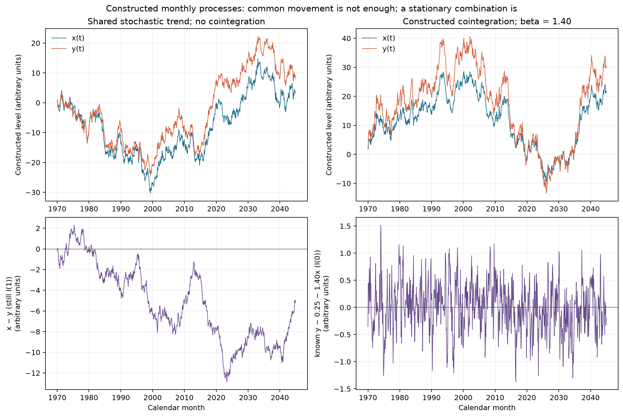
Figure 17-2: Cumulative-index proxy compounded from monthly returns for 10 French industries. The horizontal axis is the calendar month of the return observation. The vertical axis is logarithmic, after compounding the 10 industries' published monthly returns as $100\prod(1+r_t)$ and setting the displayed base for the first month to 100. The sample covers 1926-07 through 2026-08. The industries share a long-run upward movement but have different drawdowns. This is neither a single-stock price nor an out-of-sample strategy NAV; the log scale shows long-run compounding and historical drawdowns together.

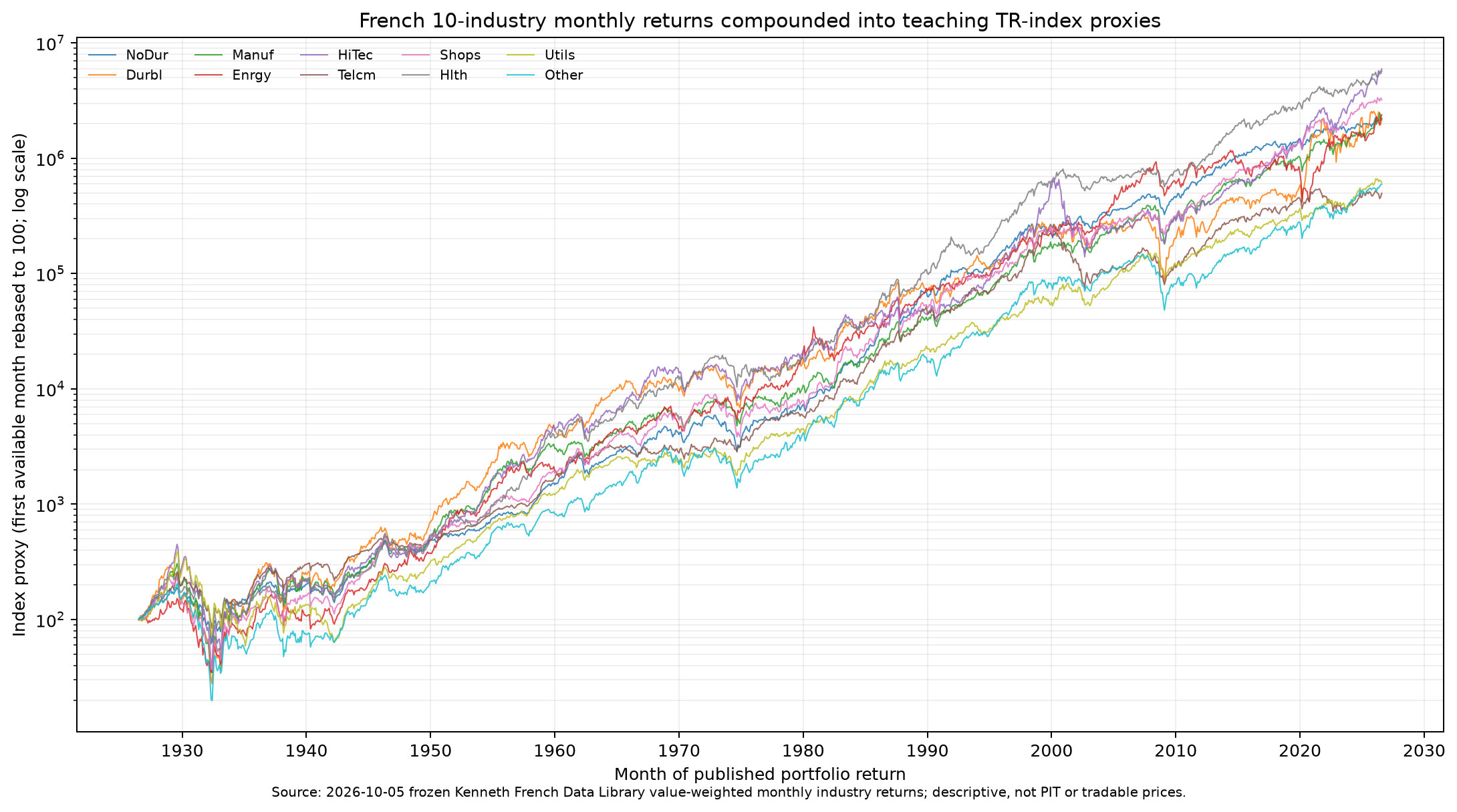
Both PNGs were generated by running code/ch17_time_series_ii.py. The code reads the local French CSV with its fixed hash and validates the legend, periods, and data range. They are not hand-drawn illustrations.

11. Real Market Example

This chapter uses the current cache of the Kenneth R. French Data Library's 10 Industry Portfolios: a ZIP downloaded on 2026-10-05, using the monthly block labeled Average Value Weighted Returns -- Monthly, with source percentages divided by 100. The source ZIP SHA-256 is ebd937a4b995d821867aeb956a96f09a666386f38fa82516b7d1767ee4a49ae5; the processed CSV SHA-256 is 3b097d810c295d64eedfa1ece7067ff2a0707f5ca90e33935df9949251f70950. The cache contains 1,202 months, 1926-07 through 2026-08. See source_notes.md and the data manifest for source-conversion details. Publicly downloadable does not mean unrestricted redistribution is licensed.

Compound each industry's published decimal simple returns into an educational TR Index proxy. During the 1926-07 through 2000-12 training interval, run a constant-term Engle–Granger test on all $\binom{10}{2}=45$ pairs; do not select trading pairs based on test-period results. The script records a minimum nominal p-value of $3.85848\times10^{-9}$, a median of 0.0516444, 22 of 45 nominal p-values below 0.05, and 15 pairs with Benjamini–Hochberg (BH)-adjusted q-values below 0.05. The false discovery rate (FDR) is the expected proportion of false discoveries among rejected hypotheses. The BH step-up procedure aims to control FDR; it does not control the family-wise error rate (FWER), the probability of at least one false positive. Its usual FDR-control guarantee requires independent tests or applicable conditions such as positive regression dependence on a subset (PRDS) of the true nulls. The pairs here share industry series, and neither their dependence structure nor the PRDS condition has been verified. The 15 BH-adjusted results below 0.05 are therefore exploratory adjusted statistics; they do not establish that FDR is controlled for this family. A small p-value does not validate future stability or imply profitability. The individual series' I(1) orders, stability across regimes, real-time data availability, and trading costs were not established by this step, so these numbers do not establish cointegration or support a trading conclusion.

These 10 columns are industry-portfolio returns, not 10 individual stocks. The cumulative values are index proxies constructed for this chapter's modeling, not executable adjusted prices for an actual fund and not point-in-time (PIT) data. The current release covers through 2026-08 and cannot reconstruct the version investors actually saw in each month since 1926. This chapter does not claim historical signal validity or report a strategy Sharpe ratio or return.

12. Common Mistakes

Mistake 1: The level correlation is 0.95, so the two series can be paired. A common stochastic trend can produce high correlation; test whether a linear combination is stationary. The output below is about 0.9552 and 0.457541; correlation is not a cointegration test.

from quant_course.cointegration import simulate_noncointegrated_common_trend, engle_granger_test
pair = simulate_noncointegrated_common_trend(n=900, seed=20261017)
test = engle_granger_test(pair["x"], pair["y"])
print(pair["x"].corr(pair["y"]), test.pvalue)

Mistake 2: Run ordinary ADF on first-stage OLS residuals and declare cointegration from the ordinary p-value. The residuals were estimated using the same I(1) data, so their null distribution differs. In the fixed simulation, ordinary ADF gives $p\approx0.23056$, while the correct Engle–Granger test gives $p\approx0.45754$. The values differ; the key point is that only the latter is calibrated for the no-cointegration null. Use this chapter's Engle–Granger interface or statsmodels coint.

import numpy as np
import statsmodels.api as sm
from statsmodels.tsa.stattools import adfuller
from quant_course.cointegration import simulate_noncointegrated_common_trend, engle_granger_test
pair = simulate_noncointegrated_common_trend(n=900, seed=20261017)
design = sm.add_constant(pair["y"].to_numpy())
residual = pair["x"].to_numpy() - design @ sm.OLS(pair["x"].to_numpy(), design).fit().params
ordinary = adfuller(residual, regression="c", autolag="AIC", result_object=True)
correct = engle_granger_test(pair["x"], pair["y"])
print(ordinary.pvalue, correct.pvalue)  # approx. 0.23056 and 0.45754

Mistake 3: Granger significance means x structurally causes y. Reversing the column order asks a different predictive question. The result concerns only incremental predictive information for the specified sample and lags. The function makes the direction explicit and checks it against a known generating direction:

import numpy as np
import pandas as pd
from quant_course.cointegration import granger_test
rng = np.random.default_rng(23)
x = rng.normal(size=1000)
y = np.zeros(1000)
for t in range(1, len(y)):
    y[t] = 0.75 * x[t - 1] + rng.normal(scale=0.5)
index = pd.period_range("1950-01", periods=len(y), freq="M", name="month")
x_series = pd.Series(x, index=index, name="x")
y_series = pd.Series(y, index=index, name="y")
print(granger_test(caused=y_series, causing=x_series, max_lag=1).pvalue)
print(granger_test(caused=x_series, causing=y_series, max_lag=1).pvalue)

Mistake 4: Estimate the relationship on the full sample, then treat old z-scores as real-time signals. Future observations change the estimated intercept and slope. Split first and estimate using only the training period. This chapter's screen_cointegration_pairs accepts only the training_end prefix; a test changes future observations and confirms that screening results remain unchanged. Real orders also require recording data availability time.

import numpy as np
import pandas as pd
from quant_course.cointegration import simulate_cointegrated_pair
pair = simulate_cointegrated_pair(n=900, seed=20261018)
train = pair.loc[:pd.Period("2000-12", freq="M")]
design = np.column_stack([np.ones(len(train)), train["x"]])
alpha_hat, beta_hat = np.linalg.lstsq(design, train["y"], rcond=None)[0]
spread_train = train["y"] - alpha_hat - beta_hat * train["x"]
print(len(train), alpha_hat, beta_hat, spread_train.std(ddof=1))

Mistake 5: Assume adjacent rows remain one month apart after dropna(). Removing a missing month makes a multi-month difference look like a one-month change. The example shows the core interface rejecting this compressed index. Trace the source or specify a missing-data model; do not fill values inside the test function.

import numpy as np
import pandas as pd
from quant_course.cointegration import validate_monthly_frame
index = pd.period_range("2000-01", periods=4, freq="M", name="month")
series = pd.Series([0.01, np.nan, 0.02, 0.03], index=index, name="return")
try:
    validate_monthly_frame(series.dropna().to_frame())
except ValueError as error:
    print(type(error).__name__, error)

13. Quant Research Application

A credible pairs study should produce an auditable chain in at least the following order.

1. State the hypothesis and falsification conditions. For example: “Two preselected assets are each I(1) in the specified regime, their log spread is stationary across multiple training and validation windows, and signal returns cover all costs.” Possible counterevidence includes different integration orders, failure to reject a unit root in the residual, relationship drift after a regime change, no out-of-sample mean reversion, or no advantage over a naive benchmark after costs.
2. Freeze the data and clock. Save source-file hashes, units, corporate actions, price/return definitions, and available_at. The industry cache in this chapter supports description of the current version of monthly portfolio returns only; it cannot give historical strategy signals PIT timestamps.
3. Split by time. Within the training interval, separately check both series' orders, specify deterministic terms, estimate long-run coefficients, test the specially calibrated Engle–Granger statistic, and account for multiple testing across families such as all 45 pairs. If screening pairs, pre-specify the candidate set and correction method; do not switch objects after seeing the validation period.
4. Freeze signals and positions. Within training, fix $\hat\alpha,\hat\beta$, spread-normalization parameters, entry/exit/stop rules, refit frequency, and each leg's dollar notional or risk budget. The cointegration regression's $\hat\beta$ is not a risk-neutral weight; define each leg's target volatility, total gross exposure, and single-leg limit.
5. Align each leg's return interval. If a signal becomes available after month t closes, do not book the full month-t return for that signal. Set the first executable time after the close, and measure both legs' next holding-period returns over the same execution interval. Monthly French published returns do not recover this execution interval, so this chapter does not calculate backtest P&L.
6. Deduct each leg's costs and compare benchmarks. Record commissions on both sides, spreads and impact, borrow availability and fees, financing, rebalancing turnover, halts/delistings, dividends, and taxes; compare with no-trade and naive hold/hedge benchmarks. Strategy validation also needs rolling or expanding windows, the available training prefix and next-period target at each step, uncertainty intervals, and crisis stress tests.
7. Audit stability and failure. Check residual ACF and structural breaks, drift in $\hat\beta$ within windows, industry-definition changes, spread tails during crises, and borrow recalls. For multiple pairs selected in training, adjusted p-values do not replace independent out-of-sample validation.

This is a research design, not a record that Project 5 is complete. This chapter has no timestamped data, execution prices, borrow records, or NAV series; it cannot claim that a pairs strategy passed out-of-sample and cost tests.

Project 5: Connecting Statistical Training Outputs to the Execution Interface

The current accepted entry point for Project 5 is projects/project05/ACCEPTED_VERSION.md, and its primary specification is preregistration v2. Its acceptance covers implementation and constructed teaching validation; real-price empirical work remains blocked. Training outputs should distinguish the long-run regression intercept and slope, Engle–Granger screening results, training-spread mean and standard deviation, and subsequent execution rules. Apply these frozen outputs at each later time point; do not renormalize using the entire future spread. If the training window changes, generate the next relationship at the pre-specified refit time rather than replacing historical fits with a future estimate.

The two chapters have distinct interface responsibilities: Chapter 16 explains the time index, effective observation count, and conditional forecast; Chapter 17 explains relationship screening and the position being held. Project 5 then calculates results using its daily trading clock, cost model, and episode definition. Passing Engle–Granger and having $\beta>0$ are only candidate-entry conditions; a trade may still not be entered or may lose money. The primary C5 constructed result, “evidence does not support this strategy,” must be retained. Do not substitute this chapter's fixed 100-dollar-notional example for the project's period-by-period share counts, actual executed notionals, and cumulative ledger. Do not upgrade the monthly French proxy into daily real trading prices.

14. Chapter Summary

First use an ADF test with the appropriate deterministic terms to ask whether the series rejects a unit root, then consider whether several I(1) variables have a stationary linear combination. Ordinary ADF and Engle–Granger tests on estimated residuals have different null distributions; the latter requires cointegration-specific critical values. A VAR links multiple variables through lags to form conditional forecasts. A Granger joint test concerns only incremental predictive power within the specified information set. Cointegration, prediction, and structural causality answer different questions; none alone establishes that trading is feasible.

For a pairs application, the key transition is from an in-sample long-run error to a real-time executable rule: estimate coefficients using past data only, trade only after the signal is available, define a common return interval for both legs, and include risk and costs in validation. Simulations help readers understand the mechanisms. The current French industry cache helps check compounding and screening counts for published returns, but does not support historical real-time trading conclusions.

15. Exercises

Attempt the exercises independently before reading the answers and derivations in Section 18.

• 17-E01 (Concept): Two random walks have a sample correlation of 0.97. Is that enough to conclude they are cointegrated? What tests or conditions are still needed?
• 17-E02 (Unit root): If $\hat\gamma=-0.08$ in the ADF regression, can you reject a unit root based on its sign alone? Explain which statistic and specification are needed.
• 17-E03 (Trend): Distinguish the persistence of shocks in $y_t=1+0.4t+u_t$ ($u_t\sim I(0)$) from that in $y_t=y_{t-1}+0.4+\varepsilon_t$.
• 17-E04 (Engle–Granger critical values): Why is it wrong to use ordinary adfuller critical values on first-stage OLS residuals?
• 17-E05 (Causality language): What does a significant result from grangercausalitytests([y,x]) test? Which stronger claim does it not support?
• 17-E06 (Model selection): What is the problem with running ADF under all three specifications c, ct, and ctt, then reporting only the smallest p-value?
• 17-E07 (Multiple comparisons): If 45 pairs each receive a 5% test, why are 22 nominally significant results not 22 verified long-run relationships?
• 17-E08 (Timing): A month-end t signal uses the full return for month t. What is wrong with calculating that signal's P&L from the same month's full return?

16. Programming Exercises

• 17-P01 (Simulation and testing): With fixed seeds, generate 900 months of a noncointegrated common-trend sample and a cointegrated sample. Report level correlations and the p-values from engle_granger_test. Acceptance criteria: the same seed reproduces the same result; the first sample has correlation above 0.9 and does not reject the no-cointegration null at 5%; the second rejects it at 1%. Label the results as simulations.
• 17-P02 (VAR time boundary): Construct a stationary bivariate monthly series. Fit a VAR(1) using only the first 80 months and forecast two months. After replacing the final 20 months with arbitrarily large values, the model input and forecasts based on the first 80 months must remain unchanged. State the output-column order, forecast months, and units.
• 17-P03 (Multiple-pair screening): Load the French 10-industry cache and compound 10 TRI proxies. Run Engle–Granger tests for all 45 pairs using only data through 2000-12; report p and BH q values. Add a constant to all post-cutoff observations and confirm that the training results do not change. Do not select pairs based on backtest returns.
• 17-P04 (Granger direction): Generate white-noise $x_t$ and $y_t=0.75x_{t-1}+e_t$, then test $x\to y$ and $y\to x$ separately. Check the column order and interpretation; do not write a structural-causality conclusion.

17. Challenge Problems

• 17-C01 (Multiple testing and selection bias): Explain how choosing the smallest-p-value relationship among the 45 pairs from 10 series distorts significance. Propose a reproducible validation plan for each rolling training window that does not revisit the selected pair out of sample. Additional prerequisites: multiple comparisons and time-series cross-validation. 10 points: record all 45 pairs (2); select within training only (2); define a correction, permutation, or testing family (2); use an independent later window (2); state falsification conditions (2).
• 17-C02 (Error correction): Starting from the cointegration error $s_t=y_t-\alpha-\beta x_t$ between two I(1) series, write an $\Delta y_t$ equation with lagged differences and explain its adjustment coefficient. Describe the long-run information lost in an ordinary differenced VAR and retained in a VECM, and how structural change can invalidate the error-correction term. Additional prerequisites: linear regression and VAR. 10 points: write lagged differences and an error term (3); explain the adjustment direction (2); distinguish long-run from short-run terms (2); give a structural-change example (2); state that this chapter does not estimate the model (1).

Additional Exercises (Independent Numbering)

• 17-N01 (Mechanism and hand calculation; §§3.1, 6.2): The common random walk has innovation variance 9, and each independent trend has innovation variance 0.25. Find the same-$t$ correlation between the two levels and the variance of $Y-X$; show that no $\beta$ can eliminate all trends. With a fixed initial level of 100 and innovations 2, −1, and 3, how do the levels change if the first shock is increased by 1?
• 17-N02 (Test diagnosis; §6.3): Explain which test interpretation to use for a pre-specified combination, same-sample OLS residuals, and new-window residuals using frozen training coefficients. Why does an ADF non-rejection in a short window with $\phi=0.99$ fail to prove a unit root? State when deterministic terms and lags should be selected.
• 17-N03 (Two-leg ledger and interpretation; §6.6): Given $K=100,d=+1,\beta=1.5$ and A/B execution prices of 20/50 and exit prices of 20.6/50.5, find share counts, gross exposure, net notional, and price P&L. Charge 10 basis points on each leg's actual execution notional at entry and exit, then find net P&L (no dividends, borrow, or financing). If $\beta=-0.5$, what direction does a long spread take? If $\beta=1.4$ and shares are rounded toward zero, what is the actual hedge ratio? Explain what it means that Project 5 excludes negative beta.

18. Solutions / Solution Hints

Exercises

• 17-E01: No. A common stochastic trend can produce high correlation without a stationary linear combination. First assess whether both series are I(1) under suitable specifications, then use a cointegration-specific procedure such as Engle–Granger to test the combination. Sample correlation provides neither critical values nor evidence that the relationship will remain stable.
• 17-E02: No. The statistic is usually an ADF t-type statistic for $\gamma=0$, with a nonstandard finite-sample Dickey–Fuller reference distribution. You also need the deterministic terms (n/c/ct/ctt), lag selection, and matching critical value. A negative slope alone is insufficient.
• 17-E03: In the first equation, under this chapter's definition $u_t\sim I(0)$ supplies only weak-stationarity and short-memory properties; those moment conditions alone do not imply a time-invariant full distribution or a vanishing response to one shock. With the additional assumption $u_t=0.5u_{t-1}+\eta_t$, a unit innovation changes the deviation by $0.5^h$ at horizon $h$, so its effect decays while the trend $1+0.4t$ is not permanently rewritten. The second equation contains a $+1$ unit root: a shock at time $t$ remains with coefficient 1 in every later level, and variance grows with $t$ under independent, identically distributed innovations with finite variance. In the two equations, 0.4 is respectively a deterministic slope and a per-period drift. The claim that the first equation's shocks are temporary depends on the additional stable causal assumption; it does not follow automatically from the definition of weak stationarity.
• 17-E04: The first stage estimates the long-run coefficient from the same nonstationary levels, minimizing the residual sum of squares. Under the no-cointegration null, that coefficient is not a stable true long-run parameter; the unit-root statistic for the estimated residual has a different null distribution from a univariate ADF test on a series specified in advance. Use the dedicated critical values returned by coint.
• 17-E05: statsmodels treats the second column, $x$, as the causing variable and the first column, $y$, as the dependent series. It jointly tests whether the specified lag coefficients of $x$ in the $y$ equation are zero. Rejection means incremental linear predictive information for the specified sample, lags, and controls; it does not show that intervening on $x$ would cause $y$ to change.
• 17-E06: Repeatedly selecting the smallest p-value implicitly includes specification search as multiple testing, so the nominal p-value no longer has its original meaning. Choose deterministic terms in advance based on assumptions about the data-generating process and report sensitivity; do not report only the most significant specification.
• 17-E07: The 45 tests can generate false positives, and the tests are dependent because they share industry series. The 22 nominally significant results describe only this exploratory family of tests. BH adjusts for FDR, and its theoretical guarantee requires independence or suitable positive dependence such as PRDS. That dependence condition has not been verified here, so 15 BH q-values below 0.05 are adjusted results, not evidence that FDR control is guaranteed; BH is not FWER control. Independent later-window testing is also needed. No adjustment guarantees relationship stability or tradability.
• 17-E08: The signal exists only once that month's return is fully formed and available. Booking P&L over the same month's start-to-end interval uses movement that occurred before the signal existed, reversing the time order. Specify the next executable time and calculate both legs' returns over the same interval after execution. Monthly portfolio files do not provide that finer-grained data.

Programming Exercises

• 17-P01: Run the chapter's core interfaces directly:

from quant_course.cointegration import (
    engle_granger_test, simulate_cointegrated_pair,
    simulate_noncointegrated_common_trend,
)
noncointegrated = simulate_noncointegrated_common_trend(n=900, seed=20261017)
cointegrated = simulate_cointegrated_pair(n=900, seed=20261018)
a = engle_granger_test(noncointegrated["x"], noncointegrated["y"])
b = engle_granger_test(cointegrated["y"], cointegrated["x"])
assert noncointegrated["x"].corr(noncointegrated["y"]) > .9
assert a.pvalue > .05 and b.pvalue < .01
print(a.pvalue, b.pvalue)  # approx. 0.457541 and 8.69312e-26

• 17-P02: The following code runs independently. First generate a stationary bivariate VAR(1), passing only the first 80 months into the fit and forecast. Then replace the final 20 months in the original panel with large values and recompute using the same training prefix. Both forecasts must be identical, begin in the month after the training cutoff, and retain the same column order.

import numpy as np
import pandas as pd
from pandas.testing import assert_frame_equal
from quant_course.cointegration import fit_var_forecast

rng = np.random.default_rng(29)
values = np.zeros((100, 2))
for t in range(1, 100):
    values[t] = np.array([0.25, -0.10]) + np.array(
        [[0.35, 0.12], [0.05, 0.30]]
    ) @ values[t - 1] + rng.normal(0.0, 0.1, size=2)
index = pd.period_range("2000-01", periods=100, freq="M", name="month")
panel = pd.DataFrame(values, index=index, columns=["A", "B"])
training = panel.iloc[:80].copy()
forecast = fit_var_forecast(training, lags=1, steps=2)

changed = panel.copy()
changed.iloc[80:] += 500.0
forecast_again = fit_var_forecast(changed.iloc[:80], lags=1, steps=2)
assert_frame_equal(forecast, forecast_again)
assert forecast.index.tolist() == [training.index[-1] + 1, training.index[-1] + 2]
assert forecast.columns.tolist() == ["A", "B"]
print(forecast)

• 17-P03: The reference implementation is located in code/ch17_time_series_ii.py, in main(): verify the frozen CSV hash; compound cached monthly returns that have already been divided by 100; set the training cutoff to 2000-12; loop over all 45 unordered pairs; calculate BH-adjusted p-values; and print every pair's unadjusted and BH-adjusted values. The core screen_cointegration_pairs function uses only the training_end prefix. A test adds 10,000 to all post-cutoff data and confirms that every result field remains the same. The reproduced counts are 22/45 nominally significant and 15/45 with BH-adjusted p < 0.05. FDR-control conditions for this family of tests on shared series have not been verified; the results do not imply 15 tradable relationships.
• 17-P04: The following code runs independently. The process makes $x_t$ white noise and sets $y_t=0.75x_{t-1}+e_t$. It tests each predictive direction on month-aligned data and asserts strong significance in the known direction, but not the reverse. Rejecting the null means incremental predictive information under the given model and sample; it is not a structural-causality conclusion.

import numpy as np
import pandas as pd
from quant_course.cointegration import granger_test

rng = np.random.default_rng(23)
n = 1000
x = rng.normal(size=n)
y = np.zeros(n)
for t in range(1, n):
    y[t] = 0.75 * x[t - 1] + rng.normal(scale=0.5)
index = pd.period_range("1950-01", periods=n, freq="M", name="month")
x_series = pd.Series(x, index=index, name="x")
y_series = pd.Series(y, index=index, name="y")

x_predicts_y = granger_test(caused=y_series, causing=x_series, max_lag=1)
y_predicts_x = granger_test(caused=x_series, causing=y_series, max_lag=1)
assert x_predicts_y.pvalue < 1e-8
assert y_predicts_x.pvalue > 0.05
print("x -> y p-value:", x_predicts_y.pvalue)
print("y -> x p-value:", y_predicts_x.pvalue)

Challenge Problems

• 17-C01, suggested argument: For each outer training window, first freeze the 10 series names, the set of 45 pairs, deterministic terms, ADF lag rule, and multiple-testing method (for example, apply BH to p-values in the training window and also report the full unadjusted distribution). Inner rolling time-series windows may compare candidates, but each outer test window evaluates only the single model selected before that window began. Do not reselect pairs or recalculate training coefficients in the outer period. When retraining for the next period, explicitly record the old and new objects. Retain failed relationships and report drift in relationship sign and half-life, out-of-sample spread ACF, each leg's post-cost returns, and confidence intervals. If a relationship exists only in one regime, one very short window, or before costs, the hypothesis is falsified. Award points according to the 5 rubric items.

• 17-C02, suggested form:

  $$\Delta y_t=\lambda (y_{t-1}-\alpha-\beta x_{t-1}) +\sum_{i=1}^{p-1}\Gamma_{yy,i}\Delta y_{t-i} +\sum_{i=1}^{p-1}\Gamma_{yx,i}\Delta x_{t-i} +\varepsilon_t.$$

  The parenthesized term is the previous period's long-run error. If $y$ is above the long-run combination and $\lambda<0$, the adjustment term lowers next-period $\Delta y$; stationarity, sign, and parameter stability still require empirical confirmation. A differenced VAR retains short-run difference dynamics but loses the level error; a VECM puts the cointegration error back into the model. If a regime change means the old $\alpha,\beta$ no longer describes equilibrium, the adjustment term can point in the wrong direction. The prompt asks for the model form and research boundary; the chapter's core code does not estimate a VECM. Award points according to the rubric.

Answers to the Additional Exercises

17-N01. The level correlation is $9/9.25\approx0.9730$, and the variance of the difference is $0.5t$. The general error variance is $t[9(1-\beta)^2+0.25+0.25\beta^2]$; the $0.25$ term keeps it strictly positive for every $\beta$, so it grows with $t$. The original levels are 102, 101, and 104. Increasing the first shock changes them to 103, 102, and 105; each later level is higher by 1, while only the first difference is higher by 1.

17-N02. For a pre-specified fixed combination, the univariate ADF reference distribution may be used under its assumptions; same-window OLS residuals require the Engle–Granger no-cointegration distribution. A new-window residual with frozen training coefficients is a stability diagnostic; training error remains, so ordinary ADF calibration is not automatically exact. With $0.99<1$, the stable AR process is close to a unit root, and a small-sample test has limited power; non-rejection means only that the current evidence is insufficient. Specify deterministic terms, the maximum lag or selection rule, and the training boundary in advance; do not search future windows and report only the smallest p-value.

17-N03. $q_A=5,q_B=-3$; gross exposure is 250 dollars and net notional is −50 dollars. Price P&L is $5(20.6-20)-3(50.5-50)=1.50$. Entry executions total 100 + 150 = 250 dollars; exit executions total 103 + 151.5 = 254.5 dollars. Total executed notional is 504.5 dollars, so the fee is $504.5(0.001)=0.5045$ and net P&L is 0.9955 dollars. With $\beta=-0.5$, $N_A=100,N_B=50$, so both legs are long. Project 5's $\beta>0$ is a strategy-screening restriction; it does not deny that general cointegrating relationships can have a negative coefficient. With $\beta=1.4$, target shares $5,-2.8$ round toward zero to $5,-2$, giving an actual hedge ratio of $100/100=1$. Recalculate risk using the actual position.

19. Further Reading

• Must Know: Dickey & Fuller (1979), pp. 427–431: focus on §§1–2 to understand the estimator distribution under a unit-root null and the deterministic-term specification. The chapter's source notes record the pages actually read.
• Must Know: Engle & Granger (1987), pp. 251–255 and 260–269: read the definitions of cointegration and error correction, the two-step estimator, and the explanation that residual tests cannot use ordinary DF critical values.
• Must Know: MacKinnon (2010), §§1–3 and the 2010 Appendix: read how cointegration-test critical values are calibrated for regressor count, trend terms, and sample size.
• Must Know: Benjamini & Hochberg (1995), pp. 289–300: focus on the FDR definition and BH step-up procedure under independent tests. Benjamini & Yekutieli (2001), pp. 1165–1188, discuss the extension under positive regression dependence on a subset (PRDS); shared industry pairs must not be assumed to meet its conditions without evidence.
• Should Know: Granger (1969), §§4–5: read the predictive meaning of “causality” and the bivariate model, noting the author's limitations concerning omitted variables, sample frequency, and nonstationarity.
• Should Know: The official statsmodels 0.15.0 adfuller, coint, VAR, and grangercausalitytests documentation: check the code API and output direction. Software documentation describes implementation; it does not replace the original theory.
• Advanced: Said & Dickey (1984), Biometrika 71(3), 599–607, on asymptotic unit-root testing when the ARMA order is unknown. For this chapter, only the OUP bibliographic record and abstract were checked; the full text was not read. See the source notes.

20. References

• Dickey, D. A., & Fuller, W. A. (1979). “Distribution of the Estimators for Autoregressive Time Series with a Unit Root.” Journal of the American Statistical Association, 74(366), 427–431. DOI. Supports the nonstandard distribution under the unit-root null in §6.1.
• Engle, R. F., & Granger, C. W. J. (1987). “Co-Integration and Error Correction: Representation, Estimation, and Testing.” Econometrica, 55(2), 251–276. Official article page and abstract. Supports the two-step estimation and cointegration-residual testing in §§5 and 6.3.
• Granger, C. W. J. (1969). “Investigating Causal Relations by Econometric Models and Cross-Spectral Methods.” Econometrica, 37(3), 424–438. DOI. Supports the predictive-causality definition and limitations in §§5 and 6.4.
• MacKinnon, J. G. (2010). “Critical Values for Cointegration Tests.” Queen's Economics Department Working Paper No. 1227. PDF. Supports the cointegration critical-value calibration in §6.3.
• Benjamini, Y., & Hochberg, Y. (1995). “Controlling the False Discovery Rate: A Practical and Powerful Approach to Multiple Testing.” Journal of the Royal Statistical Society: Series B, 57(1), 289–300. DOI. Introduces and discusses FDR; the BH procedure controls FDR under the independent-test assumption and is not a family-wise error-rate procedure.
• Benjamini, Y., & Yekutieli, D. (2001). “The Control of the False Discovery Rate in Multiple Testing under Dependency.” The Annals of Statistics, 29(4), 1165–1188. DOI. Discusses BH FDR control under positive regression dependence (PRDS); the fact that tests are correlated does not establish that its conditions hold.
• Official statsmodels 0.15.0 documentation: ADF, Engle–Granger coint, VAR, and Granger test. Supports code behavior only.
• Kenneth R. French Data Library. 10 Industry Portfolios. Supports the source and monthly data-block location for industry returns in §11; cache revision, hash, and use limits are documented in source_notes.md.