Project 6 Base Pipeline Report (A8-R1 Frozen Display)
This is not an empirical research report. Real data remain blocked. All figures below come from a constructed panel (
data_class = CONSTRUCTED) and illustrate the base pipeline's timing contract, splits, training-only tuning, portfolio rules, lagged execution, and cost ledger. The signals in the panel were specified by the author; no return or ranking is evidence about markets. A8-A's base implementation and A8-R1's display revision each have a limited-scope acceptance entry. The A8-B tree-model extension also has its own limited-scope acceptance entry. This report covers only the base layer; it does not establish that Project 6 or real-data research is complete.
1. Question and hypothesis (mechanism)
Can 46 features available at the close (3 signal features, 40 noise features, and 3 price features) be passed through a regularized linear model selected within training data to produce a dollar-neutral portfolio with positive returns after costs and outperform both the zero forecast and the training-mean baseline? In the construction, the three signal features have daily expected-return loadings of 0.03%, 0.015%, and 0.0075% per feature unit. The signal-to-noise ratio is lower than in the Chapter 39 construction.
2. Frozen design
Configuration: configs/p06_base_v1.json (read-only; SHA-256 62f49e1cab11b6992a9c391180df5d6827f9c5c12bf34f94acde5134ee4c39f7). It was frozen before any Project 6 run. Constructed results seen before the freeze (Chapters 38 and 39) are recorded in seen_before_freeze.
- Data: 40 assets and 1,512 dates starting on 2015-01-02; seed 6061. The predefined
regime_flip_at_75pctscenario reverses the signal loadings at 75% of the dates. - Timing:
signal_time = D_kclose;trade_time = label_start = D_{k+1}close;label_end = label_available_at = D_{k+6}close;h = 5. - Validation: expanding-window walk-forward grouped by date, with a 504-date initial training window and 63-date test blocks over 16 folds (first fit time: 2016-12-08). Each fold excludes 200 rows whose labels are not yet available, calculated as
. Inner selection uses two 63-date validation blocks and at least 252 training dates. Shuffled K-fold is forbidden. - Models: zero forecast, training mean, OLS, Ridge (
from through ), Lasso (5 grid values), and Elastic Net (4 × 3 grid values). Select the candidate with the lowest mean inner-validation MSE. - Portfolio: demean predictions cross-sectionally, normalize so absolute weights sum to 1, and maintain dollar neutrality. Rebalance every 5 signal dates; execute at the close of the next trading day after the signal. One-way proportional fees are 0, 10, and 20 basis points; initial cash is 1 million. NAV is marked at each daily close using the Chapter 29
run_backtest. A five-day label is not the same as a daily portfolio holding return. Borrow fees, financing spreads, market impact, capacity, and margin costs are not modeled.
3. Results (historical constructed runs)
Tables 3.1 and 3.2 retain the constructed results from the historical runs build/batches/A8-A/r1/runs/qa_r3/cli/p06_base and p06_regime. The two frozen summaries in the I3 reader package are byte-identical to the rw_qa2 summaries under qa/a8/ch37_ch39_batch/rework_r2/evidence/rw_qa2/. Compared field by field with the qa_r3 summaries, only the runtime field /seconds differs; every other summary field matches. rw_qa2 and qa_r3 have distinct run identities. This comparison does not establish that unexamined CSVs, weights, or ledgers are identical. The 13 corresponding NaN fields in each summary remain undefined and must not be read as zero.
The default P6 notebook in the I3 reader package reads frozen summaries, the display audit, and NAV images. Its actual code does not call p06_pipeline.run, retrain, or recompute daily ICs or paired dates. Older notebook prose that says it “cold-starts the pipeline from the frozen configuration” does not match its current code; the reader-mode label and actual code define it as a display replay. By contrast, running run_project06.py --data constructed ... reconstructs the panel, trains the models, and writes predictions, weights, ledgers, and summaries. That is a new run with a distinct identity. Do not describe it as the same run as the I3 replay.
The common-date audit in section 3.4 comes from a separate set of frozen daily rows and its A8-R1 display_02 evidence. Its values were not derived from the summary JSON, and must not be merged with unexamined run files as if they shared one run identity.
3.1 Base scenario
| Model | vs training mean | Mean IC (own valid dates) | t statistic shown | Own valid dates | Gross total return / Sharpe | Net after 10 bp | Net after 20 bp | Max drawdown after 10 bp | Annual turnover | |
|---|---|---|---|---|---|---|---|---|---|---|
| Zero forecast | 0 | +0.861% | — | — | 0 | 0 / — | 0 / — | 0 / — | 0 | 0 |
| Training mean | −0.868% | 0 | — | — | 0 | 0 / — | 0 / — | 0 / — | 0 | 0 |
| OLS | −1.715% | −0.839% | 0.0203 | — | 1,002 | +20.57% / 0.79 | +9.39% / 0.39 | −0.76% / 0.00 | −14.2% | 24.3 |
| Ridge | −0.982% | −0.113% | 0.0198 | — | 1,002 | +21.88% / 0.84 | +10.90% / 0.45 | +0.91% / 0.07 | −12.9% | 23.6 |
| Lasso | −0.952% | −0.083% | 0.0179 | — | 630 | +6.51% / 0.36 | −0.20% / 0.01 | −6.50% / −0.33 | −9.3% | 16.3 |
| Elastic Net | −0.879% | −0.010% | 0.0309 | — | 882 | +30.92% / 1.19 | +19.90% / 0.81 | +9.81% / 0.43 | −7.2% | 22.0 |
The test period contains 16 folds × 63 = 1,008 signal dates (about four years). The labels for the final six dates extend beyond the sample, leaving 1,002 dates in the prediction metrics.
3.2 Scenario: signal loadings reverse at 75%
| Model | Mean IC (own valid dates) | t statistic shown | Before costs | Net after 10 bp | Net after 20 bp |
|---|---|---|---|---|---|
| OLS | 0.0089 | — | +3.52% / 0.17 | −6.09% / −0.22 | −14.80% / −0.61 |
| Ridge | 0.0087 | — | +5.05% / 0.23 | −4.44% / −0.15 | −13.08% / −0.53 |
| Lasso | 0.0010 | — | −4.66% / −0.25 | −10.10% / −0.57 | −15.23% / −0.89 |
| Elastic Net | 0.0152 | — | +9.61% / 0.45 | +1.09% / 0.08 | −6.77% / −0.29 |
3.3 How to read the results
- The zero forecast beats the training mean on out-of-sample
. The training-mean baseline is −0.868% relative to zero. The historical-mean noise at the individual-stock level is large, consistent with the discussion after equation (19) in Gu, Kelly, and Xiu (2020) and section 11 of Chapter 37. The four fitted models (OLS, Ridge, Lasso, and Elastic Net) have negative relative to zero. - Keep prediction and portfolio results separate. For those four fitted models,
relative to zero is negative, while cross-sectional ICs are positive and dollar-neutral portfolios earn positive returns before costs. This is consistent with the level-versus-cross-section decomposition in section 6.5 of Chapter 38. - Costs matter. Annual turnover is about 16–24 times. At a one-way fee of 20 basis points, OLS and Lasso are negative and Ridge is near zero.
- Retain negative results. Lasso returns −0.20% after 10 basis points. In the loading-reversal scenario, OLS, Ridge, and Lasso are all negative after 10 basis points, while Elastic Net is near zero. The fold-by-fold IC figure (
p06_fold_ic_regime.png) shows negative IC in most folds after the reversal. - Tuning is unstable. Ridge's selected alpha jumps between
and across folds (the mechanism discussed in section 6.7 of Chapter 39). Lasso sets all coefficients to zero in some folds, so its IC covers only 630 dates. - Elastic Net performs best under this particular constructed setting. That result alone says nothing about real data; the same protocol would need to be run on authorized real data.
3.4 IC dates and common-date pairing (recomputed from existing frozen rows in A8-R1)
There are 1,002 candidate label dates in each scenario. Let D_m be a model's own valid-date set and
| Scenario / model | Own valid / candidate dates | Missing: constant-prediction dates | Common dates with Ridge | Model mean on pair | Ridge mean on pair | Difference in paired means |
|---|---|---|---|---|---|---|
| Base / Ridge | 1002/1002 | 0 | 1002 | 0.01982995 | 0.01982995 | +0.00000000 |
| Base / Lasso | 630/1002 | 372 | 630 | 0.01785759 | 0.01613330 | +0.00172429 |
| Base / Elastic Net | 882/1002 | 120 | 882 | 0.03087240 | 0.02060216 | +0.01027024 |
| Reversal / Ridge | 1002/1002 | 0 | 1002 | 0.00865399 | 0.00865399 | +0.00000000 |
| Reversal / Lasso | 567/1002 | 435 | 567 | 0.00100360 | 0.00308692 | −0.00208331 |
| Reversal / Elastic Net | 819/1002 | 183 | 819 | 0.01521028 | 0.00909016 | +0.00612013 |
Base Lasso and Elastic Net have 630/882 valid dates; in the reversal scenario they have 567/819. The corresponding missing counts are 372/120 and 435/183. A8-R1's frozen-row check confirmed that each of these missing dates had constant predictions. Ridge has 1,002 dates in both scenarios; OLS has 1,002 in both; the zero forecast and training mean have none. Daily and paired CSVs for all models, source hashes, and checks are under qa/a8/limited_revision_ch39_ch43_p06_v1/evidence/display_02/. This display audit did not modify the older summaries.
The A8-R1 display does not report the old IC t statistics. The old ic_summary dropped missing values and then computed NW(4) over observation indices; for a sparse daily series, a lag of four observations is not four trading days. The old values remain only in the previously accepted report and summary. A8-R1 computed no new HAC statistic and makes no claim of statistical significance. The daily series for models without missing dates was confirmed to be continuous in the original inspection, but the display removed the historical t-statistic inference throughout to avoid mixing conventions. P6 v1 and Chapter 39 are different experiments; these rows cannot be used to recompute Chapter 39's historical paired quantities.
Complete Q&A
- P6-L01 · Question: Can the base Lasso IC of 0.01785759 be compared directly with Ridge's 0.01982995 to conclude that Lasso is weaker? Answer: No paired-superiority claim follows because the models have different valid-date sets. On the common 630 dates, Ridge's mean is 0.01613330 and the paired mean difference is +0.00172429. This remains descriptive; this display provides no valid inferential t statistic.
- P6-L02 · Question: Does compressed NW(4) represent a four-trading-day HAC? Answer: No. For example, if valid trading-date indices are 0/2/3/5/8, a fourth-order lag over valid observations connects indices 0 and 8, which are eight trading days apart.
- P6-L03 · Question: Can Chapter 39 reuse these P6 paired results? Answer: No. The frozen row-level predictions needed for Chapter 39 are unavailable, so those paired values could not be recomputed. Do not retrain to fabricate historical observations.
4. Historical execution records
- The historical acceptance process checked
tests/test_p06_pipeline.py(6 tests) and the sharedtests/test_ml_pipeline.py(26 tests at c2; 34 after A8-A revision r2 added label-timing contract tests; mutation checks killed 11/11 mutants). - Historically,
run_project06.py --data realreturned exit code 3 and wrote no files. - The A8-A base notebook has a historical clean-kernel execution record. The
A8-R1/I3reader notebook is a frozen display replay and does not repeat that training. - Historical checks confirmed that every training row in each fold satisfied
label_available_at <= fit_time, and the zero and training-mean portfolios had zero turnover. These are historical acceptance records, not results newly produced for this bilingual revision.
5. Limitations and remaining work
- Real data: An authorized daily equity panel that may be retained for internal training is required (see
data_manifest.jsonfor fields and licensing). No Project 5 universe or purchase candidate is inherited. Real-data work remains blocked. - Tree models, training-only feature importance, stability, and ablation have a separate A8-B constructed-teaching implementation and limited-scope acceptance entry; see the v2 research report. This base report does not replace the separate results.
- Complete Project 6 remains unverified. BIL19 has author candidates for full bilingual teaching integration, the PCA extension, and the complete answer set; independent review is pending.
- The cost model includes proportional fees only. Borrowing, financing, market impact, and capacity are not modeled (modules from Chapters 35–36 may be connected in the complete project).
This bilingual candidate documents an existing frozen display and historical acceptance evidence. It is not new training, simulation, notebook execution, or real-data validation. Real-data work remains blocked and the complete project remains unverified; prior acceptance versions, receipts, and the frozen configuration are unchanged. The BIL19 candidates add tree and PCA teaching, stable questions P6-L04–P6-L08, complete answers, and a bilingual Loom; see the v2 guide and project-level solutions.md. The three original questions in this report are numbered P6-L01–P6-L03.
Reading the frozen constructed figures
All four frozen PNGs are retained byte for byte. They describe constructed results, supply no new significance test, and cannot fill Chapter 39's missing rows.
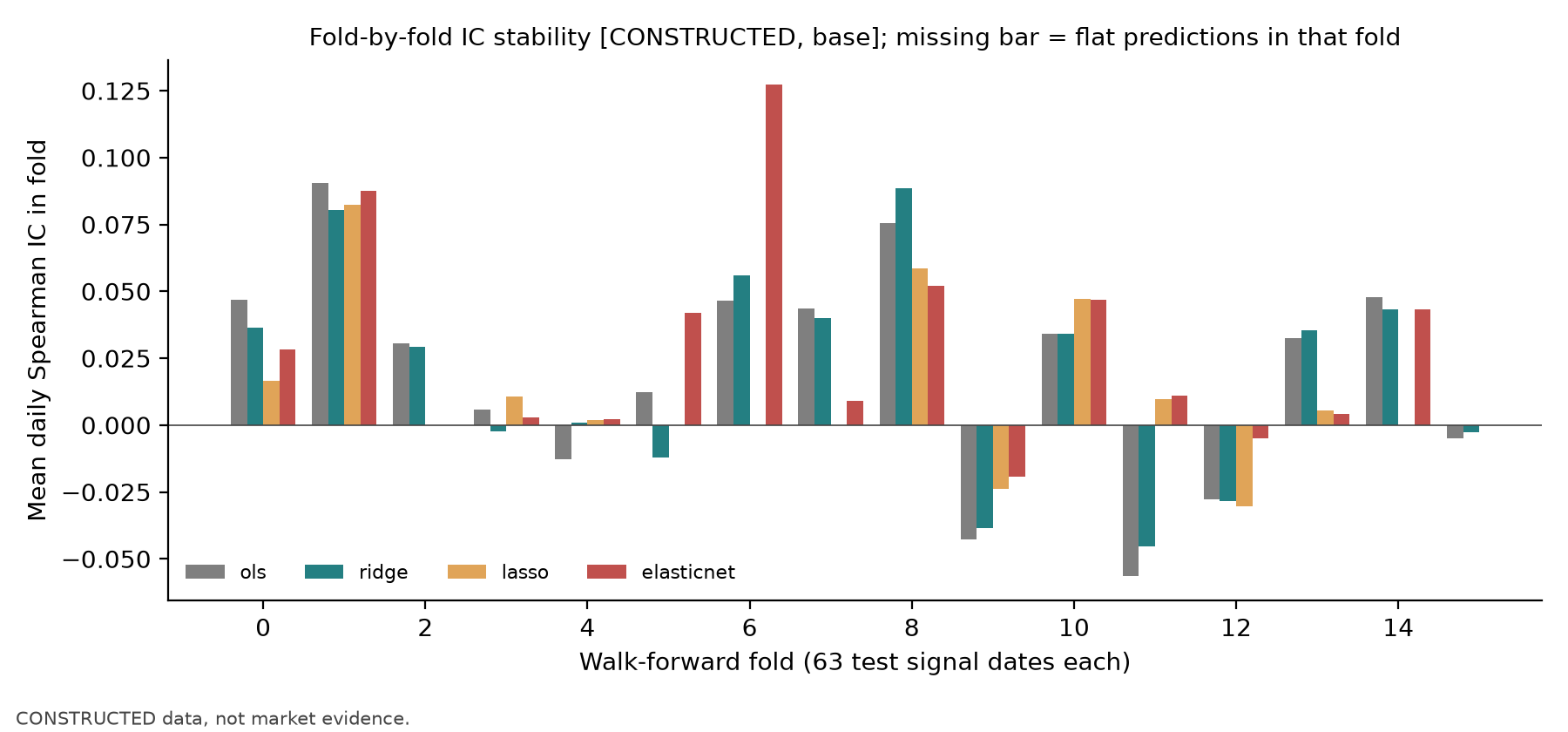
Horizontal axis: outer fold (63 test signal dates each); vertical axis: mean daily Spearman IC. Colors identify the four models; a missing bar denotes a flat predictor in that fold. Results vary across folds.
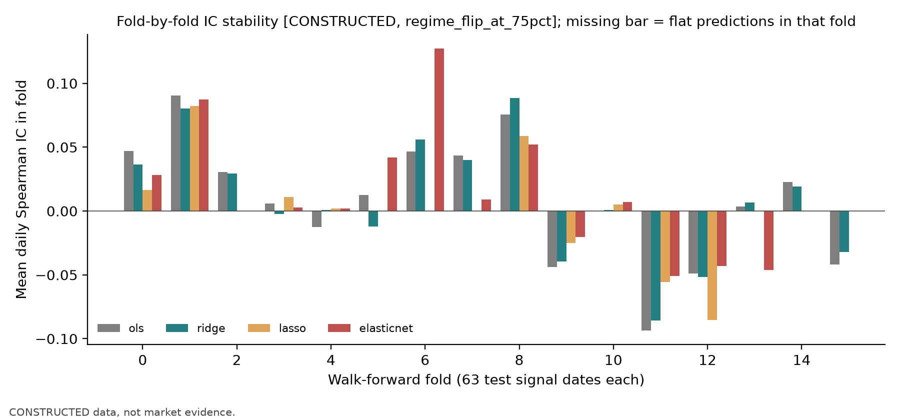
The axes and colors match the base plot. Many folds after the loading reversal have negative IC; the final positive folds do not establish general regime adaptation.
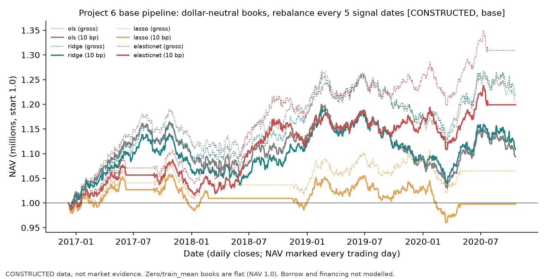
Horizontal axis: ledger date; vertical axis: NAV in millions, starting at 1.0. The legend pairs each model's gross and 10-basis-point paths; proportional fees lower wealth.
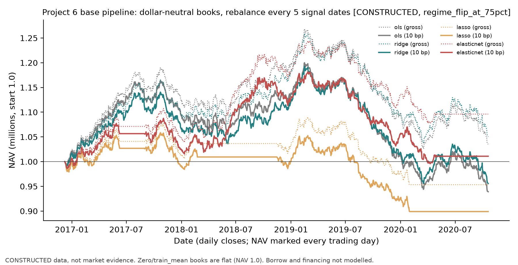
The axes and fee convention match the base NAV plot. Wealth falls after the loading reversal for several models; the full path, including losses, must be retained.