Stochastic Calculus and Derivatives

Yuxiao Ma · Advanced. Thread: start with no-arbitrage replication, build continuous pricing from available information and Itô quadratic variation, then check its boundaries through numerical results and cash ledgers.

1. Learning objectives

This chapter follows a European option from discrete replication to continuous replication, then checks analytical formulas, trees, and simulation against one another. You should be able to explain the origin of the Itô second-order term, construct a left-point integral for a specified information set, distinguish the physical measure from the pricing measure, and recompute a discrete hedging ledger with dividends and financing row by row.

The assessment actions are to calculate the stock and bond positions in one-period replication; derive the Black–Scholes PDE with continuous dividends; compute call and put Greeks in consistent units; distinguish MC sampling error, Euler discretization bias, and discrete hedging error; and use a payoff kink, an invalid tree probability, or a future-information counterexample to explain when an algorithm fails. Each action has exercises and full solutions in this chapter. Every experiment is labeled SIMULATED or CONSTRUCTED.

The level is Advanced. Prerequisites are Chapter 4 on Taylor expansions and partial derivatives, Chapter 6 on conditional expectations and normal/lognormal distributions, Chapter 9 on constraints and dimensions, Chapter 10 on contracts and payoffs, and Chapter 11 on price returns and total returns. Chapters 34–36 supply the boundaries concerning executable prices and costs. Ordinary equity alpha research follows its existing route and does not require completing stochastic calculus first.

2. Why a quant needs this

An investor forecasting next year's stock appreciation and a desk quoting a European call face different tasks. Forecasting estimates the physical distribution. No-arbitrage pricing seeks stock and cash positions whose payoff matches the option. If two portfolios have the same payoff in every model state, their current prices in an ideal market must agree; otherwise one could buy the cheaper portfolio and sell the dearer one.

A discrete tree uses two states to solve two equations. A continuous model has infinitely many paths. Adjusting the stock position to cancel instantaneous random risk requires calculating changes in functions of those paths. Brownian paths have no ordinary derivative, and the ordinary chain rule misses an accumulated second-order term. This is the concrete reason stochastic calculus enters continuous replication.

A pricing model also supplies risk sensitivities. A Delta hedger needs today's stock position, the next rebalancing time, and the cash effect of trading. A return forecaster needs the physical drift and sample evidence. Treating a risk-neutral distribution as a future-return forecast turns a pricing calculation into a purported trading signal.

3. Intuition: solve the replicating positions in two states

Teaching construction: the current stock price and European call strike are both 100. In one year the stock can only be 120 or 80; cash grows by a factor of 1.05, and there are no dividends. The option pays 20 or 0. Holding Δ shares and a current cash amount A requires both equations:

Subtracting gives 40Δ=20, hence Δ=0.5. Substitution in the down state gives A=−40/1.05. Negative cash means borrowing. In the up state, stock worth 60 minus debt of 40 leaves 20; in the down state, stock worth 40 minus debt of 40 leaves 0. Replication costs 50−40/1.05. No physical up probability is needed.

Choose an auxiliary probability p that makes the stock's expected growth factor 1.05: 1.2p+0.8(1−p)=1.05, so p=0.625. Weighting the option payoffs by this probability and dividing by 1.05 gives the same replication cost. This p comes from replication and discounting. The physical up probability could be 0.3 or 0.8 without changing the algebra. A multiperiod tree solves the replicating positions again at each node; its continuous limit becomes a predictable dynamic holding.

This tree permits only two states, no costs, and a common borrowing/lending rate. An additional independent risk state with only stock and a bond may prevent replication of every payoff. With dividends, price changes must be combined with cash received by the holder. The GBM model below retains one Brownian risk, continuous trading, and ideal financing, then checks the errors caused by discrete execution.

4. Mathematical foundations, units, and the information contract

Fix maturity T, current calendar time t, and remaining maturity τ=T−t, all measured in years. S is the ex-dividend stock price, K the strike, and V the value of an option on one share, all in the same quote currency. An actual contract multiplier is applied to the final amount; this chapter does not assume 100 shares. The continuously compounded annual risk-free rate and continuous dividend yield are r and q. Annualized volatility σ has dimension $\text{year}^{-1/2}$. Under the physical measure, μ specifically denotes the total-return drift including dividends, so the price drift is μ−q. Probability measures are $\mathbb P,\mathbb Q$; the put price is $P_{\mathrm{put}}$, or a clearly local P, to keep the two uses distinct.

Brownian increments satisfy $\operatorname{Var}(\Delta W)=\Delta t$, so W has units $\sqrt{\text{year}}$. A normal generator's scale parameter is the standard deviation: the code passes $\sqrt{\Delta t}$. Passing Δt would produce variance Δt². The return σΔW and rΔt are dimensionless, allowing the terms in an exponent to be added.

The market price of risk $\lambda=(\mu-r)/\sigma$ has units $\text{year}^{-1/2}$: μ and r have units year⁻¹, while σ has units year⁻¹/². Thus λW and λ²t are dimensionless. Δ is the number of shares per replicated option and A is a cash amount; ΔS and A can be added. Where code retains the parameter name T, API T=τ in pricing, Greeks, and MC means years remaining from valuation to maturity, rather than a calendar maturity date. The frozen example has current t=0, so numerically τ=T; its inputs are retained.

Here $f\in C^{1,2}$ means continuously differentiable once in time and twice in space. Nonsmooth payoff points at maturity are handled separately as boundaries. The call payoff $(S-K)^+$ has a kink at S=K. For T>t, the GBM Gaussian integral smooths the price on S>0; it does not make the terminal kink ordinarily differentiable.

Every strategy holding is determined at grid left endpoint $t_i$ from information then available and earns the change over $(t_i,t_{i+1}]$. Numerical hedging observes $S_i$ and rebalances immediately at that same $S_i$, an idealized simulation convention. Real-data applications must separately specify available_at, signal_time, submission, matching, and trade_time. An offline array calculation cannot establish instantaneous execution. Filtration and adaptedness below express “information then available” mathematically.

5. Formal definitions: from random paths to available information

5.1 Random-walk scaling and Brownian motion

Divide one year into N intervals, Δt=1/N, and let independent fair coins $\xi _i$ take ±1 with probability 1/2 each. Each scaled step is $\sqrt{\Delta t}\xi_i$. The N-step sum has mean 0 and variance $N\Delta t=1$. Using $\Delta t\xi_i$ instead gives terminal variance 1/N and a limit degenerate at 0; leaving steps unscaled makes variance diverge. This explains diffusion scaling. The CLT first describes the normal limit of a fixed terminal value. Weak convergence of the entire path requires a functional CLT and tightness; this chapter cites that result and does not treat the finite-dimensional CLT as its proof. A finite coin path is not a Brownian path either. [CH06_DOC_13]

Standard Brownian motion has $W_0$=0, almost surely continuous sample paths, independent increments over disjoint intervals, and $W_t-W_s\sim N(0,t-s)$. We generate paths from these increments; connecting lines merely display finite observation points. For a compatible Brownian filtration, future increments must also be independent of current $\mathcal F_s$. This chapter uses the completed, right-continuous natural filtration. Adding advance information about the future can break that premise.

The difference quotient obeys $(W_{t+h}-W_t)/h\sim N(0,1/h)$. For fixed finite M, $\Pr(|\Delta W/h|\le M)\to0$, so this family is not tight and cannot converge in probability to a finite derivative. Almost-sure nowhere differentiability is a stronger standard theorem requiring simultaneous control of all times; diverging variance alone is not its full proof. One may still take partial derivatives of a price function V(t,S), but cannot use an ordinary path velocity dW/dt.

5.2 Information, conditional expectation, and martingales

A filtration $\mathcal F_s\subseteq\mathcal F_t$ represents growing information. An adapted process has $X_t$ measurable with respect to $\mathcal F_t$. Measurability lets $X_t$ be determined from information available at t without looking at later increments. Continuous-time integration also requires suitable joint measurability, such as a progressively measurable or predictable integrand. Saying “adapted” at each time does not automatically remove those requirements.

Conditional expectation Y=$E[X\mid\mathcal F_s]$ is measurable at s and satisfies $E[Y1_A]=E[X1_A]$ for every $A\in\mathcal F_s$. In finite states it is an average with probabilities recalculated given the known state. A martingale M is adapted, has $E|M_t|<\infty$ at each time, and satisfies $E[M_t|\mathcal F_s]=M_s$ for s≤t. This is a conditional relation; a constant unconditional $E[M_t]$ is insufficient.

Make information concrete with four equally likely terminal states. Independent fair ±1 coins ξ and η are revealed in that order. Set $M_0=0,M_1=\xi,M_2=\xi+\eta$.

Strictly, $\mathcal F_{t}$ is the σ-algebra of events decidable at that time; the information groups in the table are its atoms. In finite states, $\mathcal F_{t}$-measurable means constant within every group that cannot yet be distinguished. $M_{1}$ is respectively +1 and −1 throughout the two $\mathcal F_{1}$ groups and is available at time 1. $M_{2}$ still varies within each group and cannot be used early as $M_{1}$. Conditional expectation recalculates within-group probabilities: given ξ=+1, the two states have probability 1/2 each and mean (2+0)/2=1; given ξ=−1, their mean is (0−2)/2=−1. Thus $E[M_2\mid\mathcal F_1]=\xi=M_1$; both have mean 0 under $\mathcal F_{0}$, forming a martingale. Similarly, $W_T$ contains unrevealed increments when t<T and is generally not $\mathcal F_{t}$-measurable. A value being stored in an array does not turn future information into current information.

A finite-horizon counterexample uses t=0,1,2 and a fair ±1 coin ξ: $X_0$=0, $X_1$=ξ, $X_2$=−ξ. All three means are 0. At time 1 ξ is already known, so $E[X_2\mid\mathcal F_1]$=−ξ≠ξ and X is not a martingale. Replacing the terminal value by $M_2$=ξ+η with an independent fair coin η gives $E[M_2\mid\mathcal F_1]$=ξ=$M_1$, satisfying the condition. Left-point holdings multiplied by independent future increments rely on this same conditioning step.

5.3 Quadratic variation and the domain of the Itô integral

Total variation is $\sup_\Pi\sum_i|X_{t_{i+1}}-X_{t_i}|$ over all finite partitions. For a continuously differentiable path it equals $\int|X'|dt$. Brownian total variation is almost surely infinite, while squared increments can accumulate to a finite value. Along deterministic partitions with maximum step tending to zero, Brownian quadratic variation satisfies

For the convergence needed here, $E[Q]=\sum_i\Delta t_i=T$. Independent Gaussian increments give $\operatorname{Var}((\Delta W_i)^2)=2\Delta t_i^2$, hence $\operatorname{Var}(Q)\le2T|\Pi|\to0$. Therefore $E[(Q-T)^2]\to0$, which also implies convergence in probability. Defining the quadratic variation process $[W]_t=t$ does not assert that every finite-grid QV equals t. Arbitrary path-dependent random partitions need separate treatment.

Start with a left-point simple process: $H_t=H_i$ on $(t_i,t_{i+1}]$, with $H_i$ known at $t_i$, and define the integral as $\sum H_i\Delta W_i$. For a general progressively measurable H with $E\int_0^T H_t^2dt<\infty$, approximate it by simple processes $H^{(n)}$ in $L^2(dt\times\mathbb P)$, then extend the integral to the L² limit using the isometry. For continuous H=W or the smooth path functions used here, left-point approximations meet the required conditions. An arbitrary left-point grid alone cannot establish convergence for an irregular H. [CH44_MIT_ITO]

On this domain the Itô integral is a square-integrable martingale starting at 0. In particular $E[\int HdW]$=0, and the Itô isometry is

5.4 SDEs, GBM, and the pricing model

A stochastic differential equation (SDE), $dX=a(t,X)dt+b(t,X)dW$, abbreviates an integral equation. The notation alone establishes neither existence nor uniqueness. Local Lipschitz and linear-growth conditions are common sufficient conditions. Here constant-coefficient ABM and GBM can be checked directly through explicit solutions; we do not solve arbitrary-coefficient SDEs.

The full equation, for every t, is

The second term does not first compute an ordinary dW/du and then integrate it. The dX in SDE shorthand cannot simply be separated by ordinary differential rules. The logarithmic transformation below must retain the Itô second-order term.

A European option pays $h(S_T)$ only at fixed T: $(S_T-K)^+$ for a call and $(K-S_T)^+$ for a put. Continuous replication below assumes S>0, constant r/q/σ, σ>0, one Brownian risk, no transaction costs, divisible/shortable stock, borrowing and lending at the same r, continuous predictable trading, and integrability/admissibility restrictions excluding pathologies such as doubling strategies. Numerical pricing supports T=0 and σ=0 boundaries, while the measure-change and stochastic-Greeks derivations require positive T and σ.

6. Derivations: integrals, measures, and replication prices

6.1 Why the left-point integral has a second-order correction

For any finite sequence, $a(b-a)=[b^2-a^2-(b-a)^2]/2$. Substitute a=$W_i$ and b=$W_{i+1}$, then telescope the squared endpoint differences. With $W_0$=0 this gives

This is an exact finite algebraic identity. Taking the L² limit of $Q_\Pi$ from the previous section gives $\int_0^T W_t dW_t=(W_T^2-T)/2$. For an ordinary smooth path starting at 0 the squared-increment sum tends to 0, so its ordinary chain rule has no −T/2 term. Right-point sampling instead gives $(W_T^2+Q_\Pi)/2$ and a limit larger by T. The two choices use different information and define different integrals.

The simple-process proof of the isometry expands term by term. Cross terms i<j in $E[(\sum H_i\Delta W_i)^2]$ vanish after conditioning on $\mathcal F_{t_j}$: earlier factors are then known and $E[\Delta W_j\mid\mathcal F_{t_j}]$=0. Diagonal terms are $E[H_i^2]\Delta t_i$. Their sum is $E\sum_i H_i^2\Delta t_i$. L² approximation by simple processes yields the general isometry. For H=W its right side is $\int_0^T E[W_t^2]dt=T^2/2$, agreeing with the variance of $(W_T^2-T)/2$.

6.2 Itô's formula: which Taylor terms survive accumulation?

To see the increments, first expand for sufficiently smooth functions and locally bounded coefficients, evaluating all derivatives at the left endpoint:

Second-order time terms and time-space cross terms disappear in the accumulated limit; the squared space term survives. Writing $\Delta X\approx a_i\Delta t+b_i\Delta W$ gives the square $a_i^2\Delta t^2+2a_ib_i\Delta t\Delta W+b_i^2(\Delta W)^2$. Local boundedness and grid refinement remove the first two terms; weighted quadratic variation turns the last into the integral of $b_t^2dt$. The scale $O_p(\sqrt{\Delta t})$ is probabilistic, not a common ordinary big-O bound on every path.

Why random left-point weights still permit replacement of squared increments. Fix a deterministic partition $0=t_0<\cdots<t_n=T$. Let $C_{i}$ be $\mathcal F_{t_{i}}$-measurable with $|C_i|\le K$ for one deterministic constant K. Put $\varepsilon_i=(\Delta W_i)^2-\Delta t_i$ and $R_\Pi=\sum_i C_i\varepsilon_i$. Independence of the increment from left-point information and Gaussian second and fourth moments give

For i<j, $C_i\varepsilon_i$ and $C_{j}$ are known at $t_{j}$. Conditioning on $\mathcal F_{t_{j}}$ therefore gives $E[C_i\varepsilon_i C_j\varepsilon_j]=0$. The weights need not be mutually independent: the next centered squared increment has conditional mean 0 given existing information. Consequently,

Thus $\sum C_i(\Delta W_i)^2-\sum C_i\Delta t_i\to0$ in L². Writing the second sum as $\int C_t\,dt$ still requires the corresponding process and convergence conditions for its Riemann sums. The same conditioning gives $E[(\sum C_i\Delta t_i\Delta W_i)^2]\le K^2\sum(\Delta t_i)^3\le K^2T|\Pi|^2$, while $\sum(\Delta t_i)^2\le T|\Pi|$ controls the squared-time terms. Weights that use future values do not satisfy the conditioning premise.

For the smooth functions here, stopping within a compact region bounds the coefficient/derivative weights; localization then handles leaving that region. This connects the bounded calculation to the general Itô formula, without presenting the short bound as a full remainder proof. The conclusion is for deterministic partitions and does not extend here to arbitrary path-dependent random partitions.

For $f\in C^{1,2}$, Itô's formula is therefore

The Taylor argument explains the second-order term. The general theorem for $C^{1,2}$ functions and locally integrable coefficients still needs approximation and localization to control remainders. A single o(Δt) symbol does not replace those steps. The bookkeeping rules (dW)²=dt, dt dW=0, and dt²=0 describe quadratic-variation contributions in integral limits; they are not pointwise ordinary algebra for finite random increments. [CH44_MIT_ITO, Lecture17]

For f=x², a=0, b=1, we have $f_x$=2x and $f_{xx}$=2, hence d(W²)=2WdW+dt; integration recovers the previous result. Two correlated Brownian risks require cross quadratic variation $d[W^1,W^2]=\rho dt$. The implementation here is one-dimensional.

6.3 Explicit ABM/GBM solutions, moments, and discretization error

Arithmetic Brownian motion (ABM) writes dX=a dt+b dW with local symbols a in X units/year and b in X units/√year. Direct integration gives $X_t=X_0+at+bW_t$, mean $X_0$+at, and variance b²t. Its normal support includes negative values, which violates a nonnegative-stock requirement. Applications to spreads or state variables allowed to be negative must identify their object separately.

Geometric Brownian motion (GBM) has price drift β: dS=βSdt+σSdW. Here β is a local symbol for the price drift: β=μ−q under P and β=r−q under Q. For f(S)=log S, f'=1/S and f''=−1/S². Itô's formula gives

We can also verify the candidate explicit solution backward rather than trust ordinary separation of variables. Let $F(t,w)=S_0\exp[(\beta-\sigma^2/2)t+\sigma w]$. Its derivatives are $F_t=(\beta-\sigma^2/2)F,F_w=\sigma F,F_{ww}=\sigma^2F$. Apply Itô to $F(t,W_t)$:

The exponential is strictly positive at finite t and finite Brownian values, so $S_{0}$>0 implies $S_{t}$>0. Positivity permits the logarithm and is also verified directly by the explicit solution. One may derive the logarithmic equation with stopping/localization from a positive initial value and then verify the positive solution; the −σ²/2 term missed by the ordinary chain rule cannot be omitted.

The variable $\sigma W_t$ is N(0,σ²t). For normal Y with mean m and variance v, its exponential moment $E[e^{uY}]=e^{um+u^2v/2}$ gives $E[S_t]=S_0e^{\beta t}$, $E[S_t^2]=S_0^2e^{(2\beta+\sigma^2)t}$, and $\operatorname{Var}(S_t)=S_0^2e^{2\beta t}(e^{\sigma^2t}-1)$. These supply analytical references for the terminal distribution and simulation means; they are not a single path's compounded return.

Exact grid sampling is $S_{i+1}=S_i\exp[(\beta-\sigma^2/2)\Delta t+\sigma\Delta W_i]$; Euler–Maruyama uses $S_{i+1}=S_i(1+\beta\Delta t+\sigma\Delta W_i)$. The latter factor can be negative: β=0, σ=1, dt=1, ΔW=−2 gives −100 from an initial 100, while the exact solution remains positive. This constructed counterexample diagnoses negative-price risk; it does not alter the frozen main simulation parameters.

Strong error compares paths driven by common noise. Here we estimate terminal $\sqrt{M^{-1}\sum(S_T^E-S_T^{exact})^2}$. Weak error compares expectations of a function; here g(S)=S only. We report the paired mean difference $\bar D$ and $SE=s_D/\sqrt M$. The population means of the exact and Euler solutions are respectively $S_0e^{\beta T}$ and $S_0(1+\beta dt)^N$. Higham (2001), §5 defines strong order through expected absolute error and gives Euler strong order 1/2 and, under suitable conditions, weak order 1. Our terminal L² RMSE is a different error estimator, whose numerical values must not be interchanged with that L¹ measure. [CH44_HIGHAM2001]

For linear GBM we can derive the population RMSE directly. Set h=T/N, single-step Euler factor X=1+βh+σΔW, and exact factor Y=exp[(β−σ²/2)h+σΔW]. Gaussian exponential moments and independent increments give

The terminal mean squared error is consequently

Expand each Nth power through N log(1+a h+b h²). Combining its first-order h coefficients yields the leading mean squared error term

Thus population RMSE for this GBM is O(√h). Expanding the two means in §6.3 directly gives a mean difference of O(h). Finite-grid plots show compatibility of sample estimates with these restricted analytical references; they do not prove convergence orders for arbitrary SDEs or payoffs.

6.4 From P to Q: constant coefficients over a finite horizon

Fix finite T and σ>0, with μ the total-return drift including dividends. Define λ=(μ−r)/σ and $Z_t=e^{-\lambda W_t^{\mathbb P}-\lambda^2t/2}$. This is a positive density. Gaussian exponential moments give $E[Z_t]$=1 directly, and independent future increments give $E[Z_t\mid\mathcal F_s]$=$Z_s$. Novikov's sufficient condition $E\exp[\frac12\int_0^T\lambda^2dt]<\infty$ equals $e^{\lambda^2T/2}$ for constant finite λ and T and is satisfied. The conclusion depends on those conditions. [CH44_CMU_RNM]

Girsanov's theorem gives $d\mathbb Q=Z_Td\mathbb P$ and $W_t^{\mathbb Q}=W_t^{\mathbb P}+\lambda t$. In the constant case we can also see the tilted increments: multiplying the P density of ΔW by $e^{-\lambda\Delta W-\lambda^2\Delta t/2}$ and completing the square produces N(−λΔt,Δt). Thus $\Delta W_Q=\Delta W_P+\lambda\Delta t$ is again N(0,Δt). The density factorizes over disjoint increments, preserving independence, and adding deterministic drift preserves continuity. This is a restricted verification, not a full proof for general random λ.

Substitute $dW_P=dW_Q-\lambda dt$:

The q terms cancel in λ because μ was defined as total-return drift. This change reweights probabilities on the same path space. It does not replace real investors' expected returns with r or establish known returns under P.

6.5 The correct martingales for a dividend-paying stock

Under Q, $d(e^{-rt}S_t)=-qe^{-rt}S_tdt+\sigma e^{-rt}S_tdW_Q$. For q≠0 the discounted ex-dividend stock itself is generally not a martingale; $E_Q[e^{-rT}S_T\mid\mathcal F_t]=e^{-rt}S_t e^{-q(T-t)}$. Include cash dividends in the discounted gain process:

This is a true martingale under the finite-horizon GBM second-moment conditions here. Alternatively, reinvest dividends continuously: shares $n_t$ satisfy dn=q n dt and $n_0$=1, so $n_t=e^{qt}$, wealth is $e^{qt}S_t$, and its discounted value $e^{-(r-q)t}S_t$ is also a true martingale. The two constructions use dividend cash differently; both include dividends in gains instead of ignoring the price drift.

6.6 From one-period replication to a multiperiod CRR tree

For q=0 define growth $R=e^{r\Delta t}$, stock multipliers u>d>0, and down/up payoffs $V_d$/$V_u$. Replication gives ΔuS+AR=$V_u$ and ΔdS+AR=$V_d$. Subtracting yields $\Delta=(V_u-V_d)/[S(u-d)]$; substituting into the down state gives $A=R^{-1}(uV_d-dV_u)/(u-d)$. Hence

No arbitrage requires d<R<u, making both auxiliary state weights strictly positive. The stock and bond payoff columns are linearly independent, with determinant proportional to u−d. Thus this two-state market replicates any payoff, showing how completeness appears in concrete equations.

The Cox–Ross–Rubinstein (CRR) binomial tree sets $u=e^{\sigma\sqrt{dt}},d=1/u$. Continuous dividends are explained through the reinvested total-return asset: starting with Δ shares on the left, reinvestment gives $\Delta e^{qdt}$ shares on the right. The stock contributions to the two replication payoffs are $\Delta e^{qdt}uS$ and $\Delta e^{qdt}dS$. Subtraction adds a factor $e^{-qdt}$ to the initial stock position; rearranging the initial cost yields

This establishes the dividend-adjusted forward-growth relation for the tree. Price changes alone are not the total return of a dividend-paying stock. Terminal stock values are $S_{N,j}=S_0u^jd^{N-j}$. Calculate $h(S_{N,j})$, then work backward using two-state replication at each node. Level k has k+1 nodes; update the entire level together rather than overwrite a neighbor before reading it.

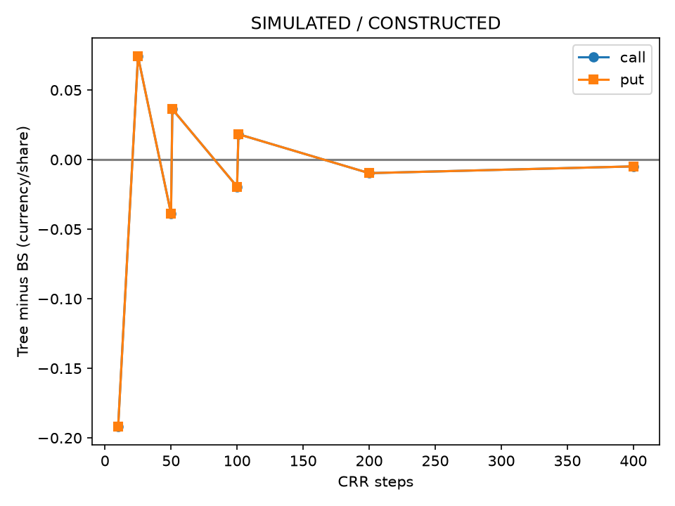
If a is not strictly inside (d,u), the two-state model fails the strict no-arbitrage requirement. Use a finer valid grid or reject explicitly. This chapter does not clip probabilities; the deterministic σ=0 boundary is handled separately. As N increases, alignment of the payoff kink with the grid changes, often producing odd/even oscillation. Smaller errors on selected grids are numerical observations, not a claim of monotone convergence for consecutive N.

6.7 Continuous self-financing replication and the Black–Scholes/Merton PDE

Replicate one European option with Δ shares and cash A, so V=ΔS+A. Self-financing means changes in Δ are paid from A with no external injection; gains arise from existing positions:

This gain equation includes dividends and financing. Applying the product rule to ΔS produces SdΔ and cross variation, which are matched by stock-rebalancing transfers in the cash account. V=ΔS+A alone does not justify treating Δ as constant indefinitely. Admissible strategies and the integral conditions here make these stochastic gain equations meaningful.

First consider instantaneous cost-free rebalancing with no interval gains. At S=100, selling 0.1 share reduces stock value by 10 currency units and raises cash by 10; ΔS+A is unchanged. The 10 is an internal transfer, not an additional gain. When the smooth pre-maturity Delta here is a semimartingale, the product formula can be written explicitly:

Adding cancels the rebalancing terms and cross variation, recovering the self-financing gain equation. Borrowed cash A accrues at the same r. Continuous dividends enter cash rather than automatically increasing shares. This expansion applies to the sufficiently smooth Delta used here; a general predictable strategy need not admit such a dΔ calculation. The general self-financing definition uses the gain integrals of existing holdings.

Under P, $dS=(\mu-q)Sdt+\sigma S\,dW_P$. Itô gives

The random coefficient in the replicating gain equation is σSΔ, so σS>0 requires Δ=$V_S$. Its drift then becomes $(\mu-q)SV_S+qSV_S+rV-rSV_S=\mu SV_S+rV-rSV_S$. Match the two drifts:

Subtract $\mu SV_S$ from both sides and rearrange to obtain the partial differential equation (PDE):

The physical μ disappears because the replicating holding cancels the same Brownian risk and its drift is constrained by financing and dividends. We have not assumed μ=r. An additional independent untraded risk, jumps, or transaction costs can invalidate the original replication equation. Merton (1973), §7, equation (44) uses remaining maturity and −$V_\tau$; converting to calendar t gives this equation. [CH44_MERTON1973]

Spatial boundaries are C(t,0)=0 and $P_{put}(t,0)=Ke^{-r\tau}$. At large S the call approaches $Se^{-q\tau}-Ke^{-r\tau}$ and the put approaches 0. S=0 is a continuous-limit boundary only; the public API requires S>0. Growth conditions and these boundaries exclude economically meaningless PDE solutions. A terminal condition alone is not a reason to ignore the solution space.

A pricing map for the same payoff. Fix $h(S_T)$, current (t,S), τ=T−t, and common financing/dividend conventions. Each layer has a different task:

Discrete hedging error on P paths checks the execution ledger within a specified model, a separate task. Q does not forecast physical stock appreciation; sharing a payoff does not imply a common P/Q drift. The next section uses bounded call/put Delta to ensure martingale conditions, with analytical verification in §6.10. The reverse route in §6.9 integrates first and checks the PDE afterward.

6.8 The Feynman–Kac link: why a Q expectation is available here

The Feynman–Kac representation connects a diffusion-generator PDE solution to a conditional expectation. Here its scope is constant r/q/σ, σ>0, positive S, finite T, continuous call/put payoffs of at most linear growth, and solutions that are $C^{1,2}$ for τ>0 with the corresponding growth and integrability.

For u∈[t,T), apply Itô under Q to $Y_u=e^{-r(u-t)}V(u,S_u)$. Its drift is the discounted PDE left side and is zero. Its random term is $e^{-r(u-t)}\sigma S_uV_SdW_Q$. Call/put $|V_S|$ is bounded by a constant depending on q and T, and finite-horizon GBM has second moments. The stochastic integrand is therefore square integrable, making Y a true martingale suitable for conditional expectation. Payoff continuity and the growth bound allow an integrable limit at T, giving

The Q-GBM Markov property makes this expectation a function of current t and S alone. A local martingale does not automatically preserve its expectation as a true martingale does; the moment conditions are part of the argument. In the reverse direction, the explicit Gaussian integral below produces a smooth price that can be checked against the PDE. No unconditional assertion is made for arbitrary irregular payoffs or degenerate/discontinuous coefficients.

6.9 Deriving calls, puts, d1, and d2 by Gaussian integration

Given current S and τ, the Q terminal value is $S_T=S\exp[m+vZ]$, where m=(r−q−σ²/2)τ, v=σ√τ, and Z~N(0,1). Exercise requires Z>−d2, where $d2=[\log(S/K)+m]/v$. Its probability is Φ(d2), and the expected strike contribution is KΦ(d2).

The stock contribution requires an exponentially weighted truncated normal integral. With φ the standard normal density, completing the square gives $e^{vz}\phi(z)=e^{v^2/2}\phi(z-v)$. Therefore

Define d1=d2+v, with m+v²/2=(r−q)τ. Discounting the stock and strike terms gives the Black–Scholes/Merton formula:

The quantity d2 supplies the Q exercise probability. The d1 term comes from exponential weighting of the stock payoff; Φ(d1) is not the unweighted exercise probability under that same Q. Delta will be $e^{-q\tau}\Phi(d1)$. The terminal call-minus-put payoff $S_T-K$, or Φ(x)+Φ(−x)=1, gives put-call parity: $C-P_{put}=Se^{-q\tau}-Ke^{-r\tau}$. The discounting relation remains valid for negative r.

6.10 Greeks: define the derivatives, then cancel repeated terms

Greeks are local risk sensitivities, with other contract parameters held fixed. $\Delta=V_S$ is replicating shares per option; $\Gamma=V_{SS}$ is the change in Delta per unit S; $\mathcal V=V_\sigma$ is currency per unit annualized volatility parameter; $\Theta=V_t=-V_\tau$ is currency/year; and $\rho=V_r$ is currency per unit continuously compounded annual rate. A first-order amount is the derivative times the parameter change. Δσ=.01 and Δr=.01 each mean one percentage point. The derivative is not an exact price change for a large shock.

Begin analytical differentiation with $Se^{-q\tau}\phi(d1)=Ke^{-r\tau}\phi(d2)$. To prove it, substitute d1=d2+σ√τ into the Gaussian density ratio: $\log[\phi(d1)/\phi(d2)]=-d2\sigma\sqrt\tau-\sigma^2\tau/2$. Substitution for d2 leaves $-\log(S/K)-(r-q)\tau$. Thus the d1/d2 chain-rule terms cancel when differentiating in S, leaving $\Delta_{\mathrm{call}}=e^{-q\tau}\Phi(d1)$. Put Delta follows by subtracting $e^{-q\tau}$ via parity. Differentiate once more using $\frac{\partial d1}{\partial S}=\frac1{S\sigma\sqrt\tau}$ to obtain Gamma.

Differentiating in σ makes the two CDF chain terms a common density coefficient times $(d1_\sigma-d2_\sigma)=\sqrt\tau$, giving $\mathcal V=Se^{-q\tau}\phi(d1)\sqrt\tau$. In the r derivative, $\frac{\partial d1}{\partial r}=\frac{\partial d2}{\partial r}=\frac{\sqrt\tau}{\sigma}$, so the chain terms cancel and leave the strike-discount derivative. Theta follows from substituting Delta/Gamma into the PDE to obtain −$V_\tau$, or by differentiating directly in maturity. The results are

The PDE provides a scenario-by-scenario check: $\Theta+(r-q)S\Delta+\sigma^2S^2\Gamma/2-rV=0$. Call and put Theta can have different signs; time decay need not be negative for every parameter choice. Central differences use (V(x+h)−V(x−h))/(2h), and Gamma uses a second difference divided by h². Calendar Theta negates the remaining-maturity difference. Finite h causes truncation error; overly small h amplifies rounding through cancellation. Left/right derivatives differ at the maturity kink. This API rejects all T=0/σ=0 Greeks, while the documentation explains that deterministic derivatives away from the kink are unimplemented.

6.11 Monte Carlo under Q and antithetic variates

This subsection shifts the current valuation time to 0. Its T is the shifted remaining maturity, namely τ=calendar maturity−current time on the original clock. The terminal subscript T below uses that shifted clock, and API T also equals τ. At an arbitrary current t, one must not pass the unadjusted calendar maturity to MC.

Monte Carlo (MC) draws independent $Z_i$ and uses exact Q terminal values $S_T^{(i)}=S\exp[(r-q-\sigma^2/2)T+\sigma\sqrt T Z_i]$ with discounted payoffs $Y_i=e^{-rT}h(S_T^{(i)})$. A European payoff depends only on the terminal value, so exact sampling removes Euler time-discretization bias. Finite random samples retain sampling error. The estimator is mean(Y), with $SE=s_Y/\sqrt M$. For finite variance and sufficiently large M, the normal approximation gives 95% CI=mean(Y)±1.95996398454SE; this is not exact finite-sample coverage.

Antithetic variates use each independent $Z_i$ to generate both $Z_i$ and −$Z_i$, with $X_i=(Y_i^++Y_i^-)/2$. The M values $X_i$ are independent across pairs; the two payoffs within a pair are correlated. The correct SE is $s_X/\sqrt M$, with $\operatorname{Var}(X)=[\operatorname{Var}(Y^+)+\operatorname{Var}(Y^-)+2\operatorname{Cov}]/4$. Antithetic correlation for the monotone vanilla payoffs here usually reduces variance; this numerical conclusion is not extended to every payoff. At the same number of independent observations, antithetic sampling uses twice as many terminal-payoff evaluations. Cost comparisons must state this.

The typical SE scale as sample size grows is $M^{-1/2}$; the realized pricing error in a particular batch need not decrease monotonically. One analytical price falling inside a CI is one random outcome. Analytical/financial identities, independent formula checks, and boundary rejection jointly assess algorithm correctness. A random sample with M=1 cannot estimate s². Only deterministic σ=0/T=0 cases directly return SE=0 and a point interval.

6.12 A discrete Delta-hedging ledger: who receives cash each interval?

Simulate the P price drift μ−q with initial capital $V_0$ equal to the Q model price. Buy $\Delta _0$ shares, leaving cash $A_0=V_0-\Delta_0S_0-\mathrm{fee}|\Delta_0|S_0$. Initial purchase costs are deducted from the capital rather than financed by an unreported injection.

Let dt=T/N. Hold the previous post-rebalance shares $\Delta _{i-1}$ and cash $A_{i-1}$ fixed. Before rebalancing at the next endpoint, cash follows the protocol's approximate recursion:

Continuous-model cash dividends are $\int q\Delta S_u\,du$. This recursion approximates interval dividends using the left-point price and fixed old holdings, and books all interval cash flow at the right endpoint. It omits differing financing times for dividends received within the interval. This discretization differs from the continuous formula. Exact sampling of S terminal values does not make the whole hedging ledger exact continuous replication.

Observe $S_i$, compute the new Delta with remaining maturity $T-t_i$ for the following interval only, and trade $\delta\Delta=\Delta_i-\Delta_{i-1}$. Cash becomes

At maturity force $\Delta _N$=0 and deduct liquidation costs. Final error is $A_N-h(S_N)$. Both cash and shares must reconcile. Negative cash A accrues financing at the same r; the simulation has no real borrowing/lending spread. The sum $\sum\mathrm{fee}|\delta\Delta|S$ is nominal cash fees only. Their effect on terminal funds also includes financing opportunity cost, so the difference in mean errors across frequencies cannot simply be equated to mean fees.

7. Financial Interpretation: Prices, Probabilities, and Hedging Cash

Stock price changes must be distinguished from total stock returns. Holding Δ shares produces dividend income of ΔqSdt; the borrowing balance accrues interest at rate r. If dividends are omitted from the replication ledger, the stock term in the PDE is incorrectly written as r instead of r−q, and call and put prices and Deltas will then be inconsistent. Two pricing algorithms can be compared only when they use the same payoff, financing, and allocation of cash flows.

$\mathbb Q$ is a measure consistent with the model's no-arbitrage assumptions. In the complete-market model used in this chapter—one Brownian source of risk, a stock and a cash account, σ>0, continuous trading, and suitably integrable strategies—a replicable European payoff has a unique model price. Completeness means that every admissible payoff can be replicated with tradable assets; with no arbitrage but an incomplete market, the price need not be unique. The case σ=0 is a deterministic boundary, so the conversion formula based on the market price of risk λ=(μ−r)/σ cannot be applied directly.

Monte Carlo pricing computes expectations under Q. The discrete hedging experiment instead sets μ=.08, including dividends, under P to examine the error along the specified model paths. The two experiments share r, q, σ, and the payoff, but differ in purpose, measure, and drift. Hedging error is defined as the cash remaining after liquidation minus the option payoff. A positive value means the replicating portfolio has excess cash; a negative value means it is short of the required cash. This is not the investment return from holding one option.

Frictionless continuous replication provides a model benchmark. Discrete rebalancing leaves Gamma risk, and approximating dividends and cash flows over intervals introduces error. More frequent rebalancing also increases fees. The 10 bp fee is a constructed input; it has not been checked against order-book quotes or estimated market impact. Connecting the hedging chart to real profitability would still require validation of quotes, latency, borrowing, jump risk, and data permissions.

8. Numerical Example: Frozen European Pricing and Hedging Experiment

All results are SIMULATED / CONSTRUCTED, with each payoff corresponding to one share. Inputs are $S_0$=K=100, T=1 year, r=.05, q=.02, and σ=.20. The protocol was fixed before the first run; the historical output was originally in build/batches/A9-A/r1/runs/experiment_output_02 and has since been archived. Original run identities are recorded in the archive inventory. The numbers below retain the accepted historical independent root run; its existing results.json is available separately. The existing root results and archived author run retain distinct identities. This bilingual batch neither reran the experiment nor extracted the archive. All amounts are per-share teaching amounts in the same currency.

8.1 Intermediate Values for the Hand Calculation and Analytic Price

For the one-period tree without dividends, the replicating position is .5 shares and cash of −38.0952380952, giving a price of 11.9047619048. The up-state payoff is 20, the down-state payoff is 0, and the auxiliary probability is p=.625, matching the equation in §3. Its multipliers 1.2/.8 and growth factor 1.05 differ from those of the main CRR grid, so the difference between their prices must not be called an algorithm error.

For the main example, log(S/K)=0, (r−q+σ²/2)T=.05, and σ√T=.2, so d1=.25 and d2=.05. The discounted stock amount is $100e^{-.02}=98.0198673307$, and the discounted strike is $100e^{-.05}=95.1229424501$. Multiplying each by its respective CDF and taking the difference gives a call price of 9.2270055082 and a put price of 6.3300806275. The parity difference is 2.8969248806, with a calculation residual of 0 within double-precision range. This identity checks dividends and discounting more directly than a single simulation interval covering the price.

8.2 CRR and Analytic Price Comparison

The 25/50/51 and 100/101 grids show the effects of parity and payoff-grid alignment. Call and put errors overlap in the chart because of parity in this model. Valid probabilities are rechecked as the step size changes; connecting lines are only for reading adjacent choices. No claim of monotone convergence is made.

8.3 Exact Terminal-Value Monte Carlo under Q

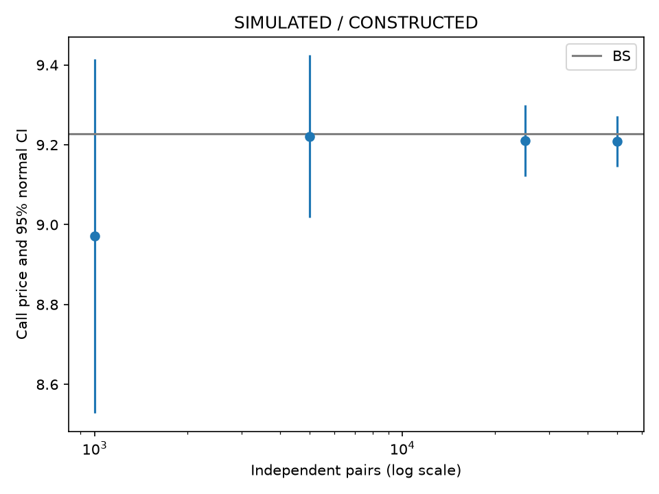
Seed 4401. For antithetic sampling, the independent unit is the pair mean. Each row uses M independent pairs and 2M terminal payoff calculations; the 95% interval is a normal approximation.

For 50000 ordinary independent paths, the call SE is 0.061862; for the same number of independent pairs, the SE is 0.032531. The number of payoff calculations differs, so this is not a comparison at equal computational cost. A single interval covering the analytic price does not prove the algorithm is correct, and the error need not decrease monotonically each time M increases.

8.4 Finite-Grid Brownian Quadratic Variation and Its Limit

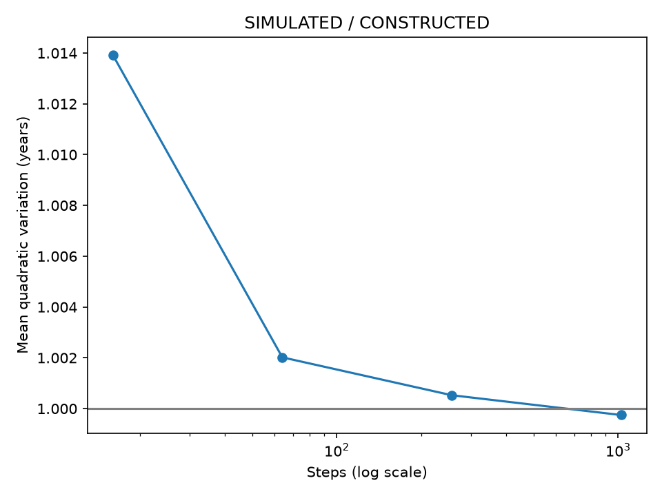
Seed 4402, with 1024 fine increments on each of 1024 paths, aggregated into nested grids; T=1.

Each finite identity uses the actual QV for that row; only the last column replaces QV with its theoretical limit T. The sample means and SDs are compared with the theoretical values $E[QV]$=1 and Var(QV)=2/N. The numerical pattern for this seed and these grids is not a general proof for all partitions or paths.

8.5 Exact GBM and Euler under P with Shared Increments

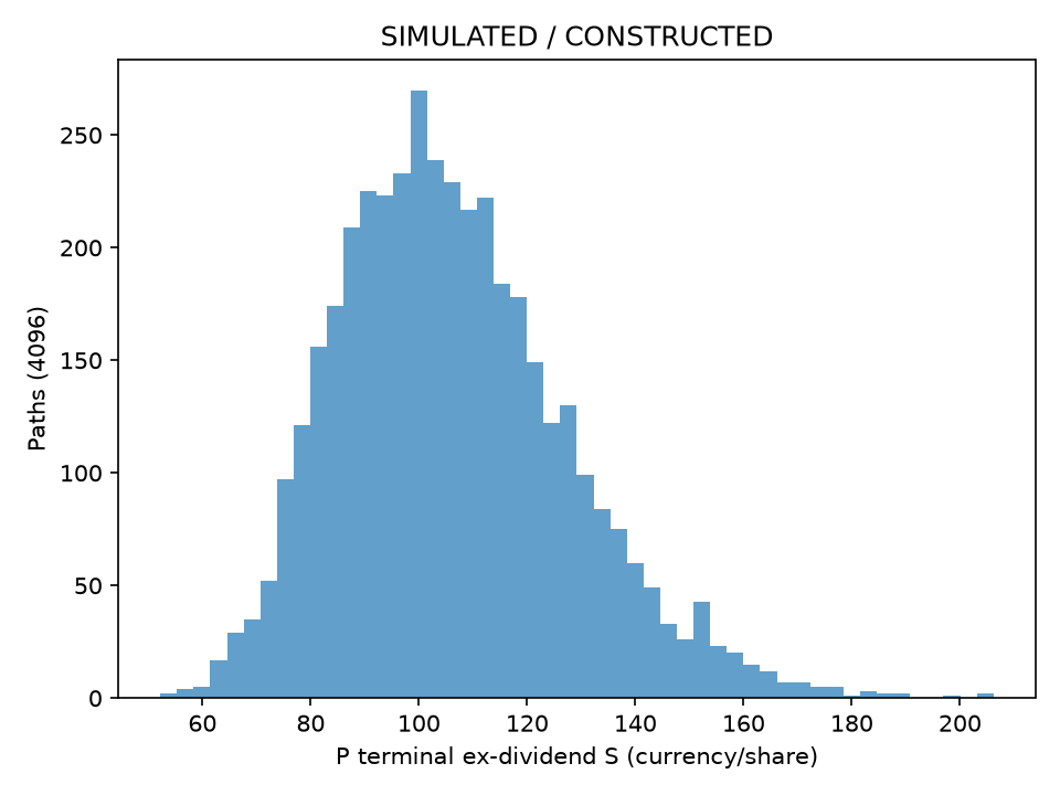
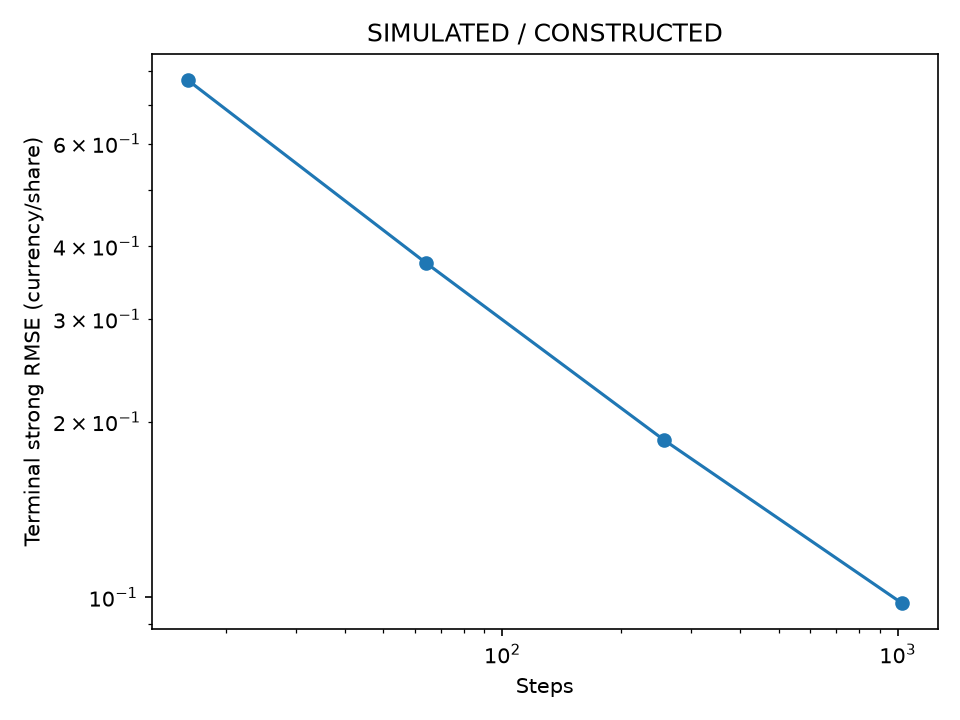
Seed 4403, with 4096 fine paths, dividend-inclusive μ=.08, and stock-price drift .06. Strong error uses the terminal difference D along the same Brownian path; the weak difference is the signed mean(D), and the paired SE is reported.

The strong-error scale on finer grids is consistent with Euler's strong order 1/2. The weak sample difference is larger at 1024 steps than at 256; the paired SE explains why monotonicity is not required. For the exact model, $E[S_1]$=106.183655; moments and the terminal distribution are given in §6.3. No negative Euler prices were observed on these grids, which describes only this sample; the separately constructed example with dW=−2 still produces a negative Euler price.

8.6 Greeks and Step Size

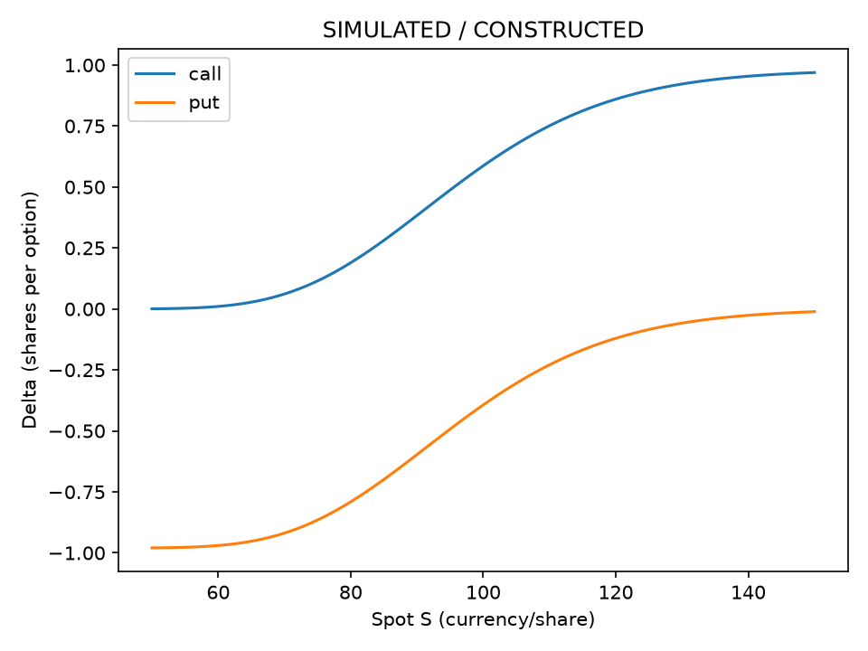
Vega and Rho are reported per unit parameter change; Theta is per calendar year. Centered differences were checked for calls and puts at S=80/100/120 with other inputs fixed. The maximum absolute error across different units is only an execution summary of per-item tolerances; it should not be treated as a single economic distance.

For every scenario and metric, the absolute centered-difference error is below 2.2e−6 in its own units, with h=.0001 and stock-price step $h_S=S\cdot h$. The base call Vega is 37.9011575100, so a 1 pp volatility shock has a first-order price effect of approximately .3790115751. The put Theta at S=80 is positive, so it is not valid to claim that time always erodes every option's value.

The very small h=1e−8 has already lost accuracy; the source code retains this negative diagnostic.

8.7 Discrete Delta Hedging under P and Fees

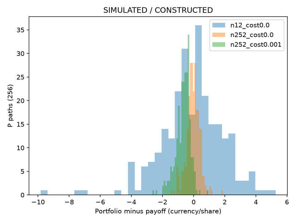
Seed 4404, with 256 shared Brownian paths of 3276 fine steps, aggregated to 12/52/252 steps. The P stock-price drift μ−q=.06 is distinguished from the Q pricing drift .03. fee=.001 is a one-sided 10 bp fee, charged at initiation and liquidation; amounts are per share.

Without fees, higher frequency lowers the error SD in this sample. With fees, higher frequency produces a more negative mean and larger average fees; the 95th percentile is also negative at 252 steps. This comparison retains replication shortfall and fees and does not promise real-world profitability at any frequency. The difference in mean error includes fee financing drag; total fees are a nominal sum.

8.8 Cash and Share Reconciliation in a Complete Ledger

Path 0, 12 steps, fee=.001, with time i/12 years. The tables separate cash flows on the old position from the current rebalance. Unrounded values from the existing independent root run are in ledger_n12_cost0.001.json; the archived author payload is separately indexed above. Use the actual floating-point values to reconcile the ledger with the code in §18 rather than requiring 1e−10 agreement from six-digit displayed values.

Initial cash equals the model price minus the stock purchase and initial fee. Over each interval, the carried share position receives dividends. On the final row, the share count and stock market value are zero, and liquidation cash minus payoff is the path error. Cash fees and financing costs reduce replication funds even when the terminal stock path is unchanged.

9. Python Implementation

Throughout this section, the public pricing parameter T denotes remaining time to maturity τ, in years. For example, if calendar time t=.25 and maturity $T_{\mathrm{maturity}}$=1, pass T=.75 to the API. Theta remains the calendar-time derivative −$V_\tau$; its sign does not change because the API parameter is named T.

Core calculations are in src/quant_course/stochastic_calculus.py and derivatives_pricing.py, and are reused by the CLI and Notebook. Run the CLI from the course root using the existing .venv. All prices are in currency per share. The output directory must not already exist; if a run fails, retain that directory and continue with a new path.

.venv/bin/python code/ch44_stochastic_derivatives.py \
  --output-dir runs/reader_01
.venv/bin/python -m pytest \
  tests/test_stochastic_calculus.py tests/test_derivatives_pricing.py \
  tests/test_ch44_root.py -q

The CLI records fixed seeds, Monte Carlo pricing under Q and hedging under P, analytic/tree errors, Greek finite differences, shared Brownian increments, error estimators for every grid, figures, and one complete cash ledger. Run the Notebook from a clean kernel in first-cell order; it calls the core functions and generates PNGs during execution. Its smaller demonstration does not replace the full frozen CLI experiment.

Public pricing functions reject NaN, infinity, non-positive S/K, negative σ/T, and invalid call/put types; r may be negative. The tree rejects invalid probabilities rather than clipping them to 0 or 1. Prices at expiry and at zero volatility use the deterministic payoff. The Greeks API supports T>0 and σ>0; it explicitly rejects inputs at expiry or with zero volatility. At the payoff kink there is no ordinary unique derivative, while some deterministic derivatives can exist away from the kink; this API does not provide them. If extreme parameters exceed floating-point range, the function should raise a clear error rather than return a seemingly valid NaN.

The left-point integration function checks dimensions, shapes, and finite values; it cannot infer the information source of a numerical array. The caller is responsible for proving the integrand is adapted. The GBM function's drift is directly the stock-price drift: pass μ−q=.06 under P or r−q=.03 under Q; the function does not subtract q again.

10. Visualization

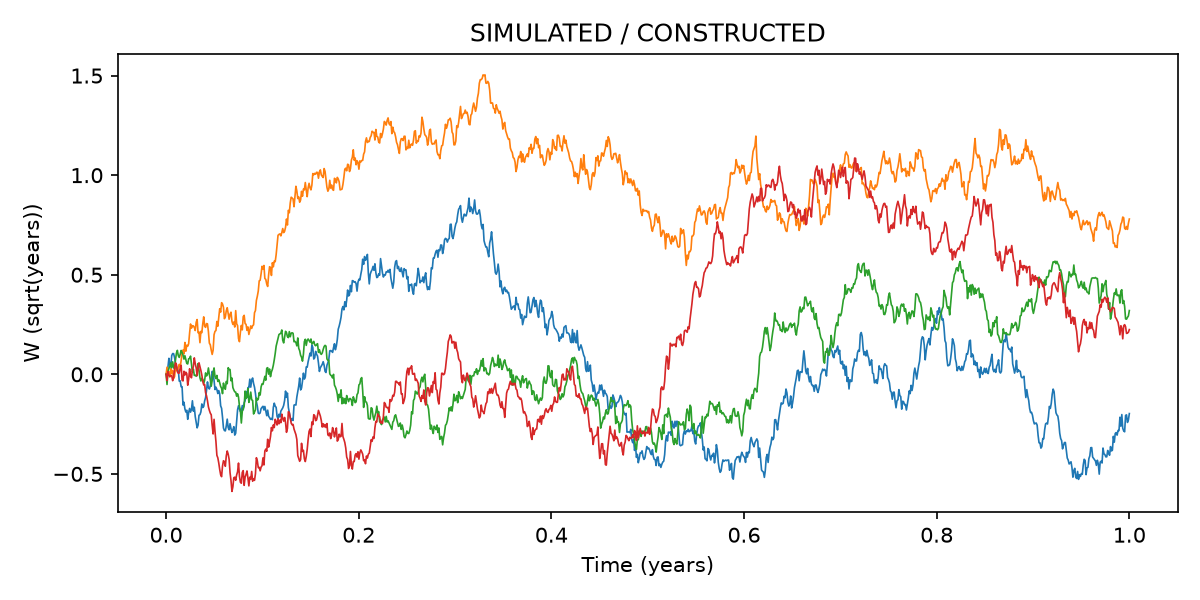
The eight generated figures are placed beside the corresponding numerical results in §8, so reading the charts stays connected to the calculations. Inputs, units, random seeds, and sample sizes are described with each figure; the SIMULATED label appears on the charts. Brownian connecting lines do not imply smooth paths, the gray QV line is the population limit, tree-error connecting lines do not imply monotonicity, Monte Carlo error bars are sampling intervals, the Delta curve shows local model sensitivity, and the hedging histogram is under P rather than Q.

The figures can be rebuilt by the standalone CLI in a new directory; retain the output results together with the PNGs.

11. Real Market Example: A Testable Question from the Model

This chapter did not download a real option chain or report real market quotes and model-price differences. Agreement among the three pricing methods inside the model therefore checks only the numerical implementation and the relationship under the stated assumptions. With permission to use the data, you could ask a vendor a practical question: for the same underlying, expiry, strike, currency, timestamp, bid/ask quotes, and dividend curve, compute the implied volatility for each valid quote and test whether a single constant σ can explain them.

A volatility smile or skew means that implied volatility varies with contract characteristics such as strike. It is a pattern in model parameters backed out from prices, not an observed return distribution under the real-world measure, and it cannot be directly interpreted as trading Alpha. Before inverting mid-prices, check the bid/ask range, payoff convention, and dividends. If a constant-σ model shows systematic differences across many strikes, stochastic volatility, local volatility, or jump models may be needed; their hedging performance would still need to be tested.

The original Black–Scholes paper assumes no dividends and no transaction fees; Merton's dividend extension supports the q term in this chapter. Those theoretical sources do not mean that this chapter replicated their market studies. The real-market example remains pending validation with licensed data. Missing evidence includes quote URLs and permissions, download date and version, sample period, synchronized quotes and execution latency, currency-consistent rates and dividends, hashes, and reproducible cleaning. This chapter does not invent a volatility surface or market prices to fill that evidence table.

12. Common Mistakes: Runnable Counterexamples for Diagnosis

Mistake 1: Treating a Brownian path as an ordinary smooth path and calculating $\int WdW=W_T^2/2$, thereby omitting half the quadratic variation. On a finite grid, the correct value is $(W_T^2-\sum\Delta W^2)/2$, whose limit is $(W_T^2-T)/2$. The incorrect and repaired code in 44-P01 returns the difference between the two, instead of merely saying “remember randomness.”

Mistake 2: Copying the terminal value $W_T$ to every left endpoint as the integrand. The program can multiply the values, but the integrand uses future information; the resulting terminal sum is $W_T^2$, with expectation T, unlike the zero expectation of an adapted, square-integrable Itô integral. Correct array shape does not fix look-ahead. Perturbing a future suffix provides negative evidence about one code path's information dependence, but finite tests cannot prove that every input is adapted.

Mistake 3: Replacing r−q under Q with μ−q under P and then discounting at r. This computes a discounted expectation under P and generally does not replicate a European payoff. 44-P03 computes both the correct Q model and the incorrect drift construction for comparison; the role of Q follows from the model's assumptions of σ>0, completeness, and no arbitrage.

Mistake 4: Calculating the SE for correlated antithetic paths as though there were 2M independent samples. In 44-P04, both payoffs are generated from the same z and averaged within each pair first; the correct SE comes from the sample variance of the M pair means. The direction of error in the incorrect SE depends on payoff correlation; this chapter's example must not be stated as a theorem that antithetics reduce SE for every payoff.

Mistake 5: Treating Vega itself as the price change for a one-percentage-point volatility move, or treating Theta with respect to remaining time as Theta with respect to calendar time. 44-P04 provides centered differences in matching units and the 1 pp conversion. A step size that is too small can make Gamma inaccurate through cancellation; one that is too large introduces truncation error. More displayed decimal places do not guarantee greater accuracy.

Mistake 6: Recording only stock rebalancing in the hedging ledger, omitting interest on existing cash or dividends on the existing stock position, or retroactively crediting past dividends using the new Delta. 44-P05 recomputes the old position's interval cash flows, current rebalance, and initial and liquidation fees row by row; it also shows the difference between the incorrect and correct ledgers. Using a future Delta or omitting fees changes the financial task.

13. Quant Research Application: From Model Checks to a Data Experiment

A research question could be: “Does increasing discrete hedging frequency reduce replication-loss risk after fees?” First fix the underlying/payoff and the sign convention for the error. Use frictionless continuous replication as the benchmark, then freeze the candidate frequencies, one-sided fee, P-path parameters, sample size, and seed. This chapter first examines sensitivity inside the model and retains the mean, SD, percentiles, and fees. A smaller error under one seed does not show that another market environment will behave better.

For real data, split the timeline into an estimation period for volatility, dividends, and fees, and a later period that is evaluated only once. This ensures every hedge uses only information available at that time. Record each bid/ask and execution eligibility, cash rates and borrowing spreads, settle the same fixed payoff, and compare with simple baselines such as no hedge, fixed Delta, and low-frequency Delta. Report pricing error, hedging risk, and net trading-strategy return separately.

Specify possible disconfirming outcomes in advance: a constant σ cannot explain the quote range; jump or tail replication shortfall exceeds the risk limit; fees from higher frequency offset the error reduction; or synchronized/licensed data are insufficient for reproduction. Any of these could prompt a revision to the model or execution assumptions. If parameters are changed after viewing the later period, label the analysis post hoc rather than rewriting it as preregistered. The results in this chapter deliver only the simulated teaching candidate described above, not a completed real-derivatives project acceptance.

14. Chapter Summary

The two-state replication equations give the risk-neutral probability; the information set constrains usable dynamic positions; Brownian quadratic variation explains the second-order Itô term; and GBM combines these conditions into a positive-price path. Continuous self-financing replication eliminates the real-world drift and leaves a PDE involving r, q, and σ. The risk-neutral conditional expectation connects the analytic solution to numerical methods.

In practice, first check the payoff and units, then the model and information conditions, and then choose the analytic formula, tree, or Monte Carlo method. Check Greeks with finite differences, calculate SE using the independent sampling unit, and check hedging error with a complete cash ledger. Numerical agreement supports the implementation; real quotes, costs, and jumps still determine the model's application boundary.

15. Exercises

44-E01: Scaling and the Scope of the Proof

For a fair-coin random walk over one year with N steps, let the step size be either ξ/√N or ξ/N. Find the terminal variance in each case. What distribution does a Brownian difference quotient follow? Explain why this rules out a finite derivative in probability at a fixed time, and why it does not by itself prove almost-sure nondifferentiability everywhere. Derive the expected QV and its variance bound for a deterministic grid.

44-E02: Zero Unconditional Mean Does Not Imply a Martingale

Let ξ be fair ±1 and define $X_0$=0, $X_1$=ξ, $X_2$=−ξ. Write the three means and $E[X_2\mid \mathcal F_1]$, then determine whether X is a martingale. Next change $X_2$ to ξ+η, where η is an independent fair ±1, and determine whether it is a martingale. Besides adaptation at each time, what measurability and integrability conditions does a continuous Itô integrand require?

44-E03: Finite Grid and Limit

For the path W=[0,.2,.1,.4], calculate the sum of squared increments, the left-point sum, and the right-point sum. Use telescoping sums to derive the general expressions for both sums. For Brownian motion with T=1, explain which equality holds only in the limit when QV is replaced by 1.

44-E04: GBM and Common Noise

Under P, let μ=.08, q=.02, σ=.2, and $S_0$=100. Find the stock-price drift, log-price drift, $E[S_T]$, Var($S_T$), and their expressions at T=1. Derive the Euler recursion and give a negative-price counterexample. Write the strong terminal RMSE and the paired estimator for the weak error with g(S)=S. Must the weak error be monotone across grids?

44-E05: Measure Change and Dividend-Adjusted Martingales

With the same parameters and r=.05, find λ, $Z_t$, $W_Q$, and the Q stock-price drift. Show that Novikov's condition holds over a finite horizon, then write the drift of the discounted ex-dividend price, the discounted return process including cash dividends, and the wealth process with dividends reinvested. Explain why the λ formula cannot be used when σ=0.

44-E06: One-Period Replication

Let $S_0$=K=100, $S_u$=120, $S_d$=80, the bank-account growth factor be 1.05, and q=0. Find the replicating share position, initial cash/bond position, call price, and auxiliary risk-neutral probability; check both states. How does the replication price change if the real-world probability of an up move is .3?

44-E07: Self-Financing and the PDE

Starting from V=ΔS+A, the dividend-financing flow in dA, and Itô's formula for dV, derive the PDE including q term by term. Explain why applying the ordinary product rule directly to ΔS would incorrectly treat rebalancing as an external contribution. State the European call/put terminal payoff and the σ>0 domain, as well as the borrowing and trading assumptions.

44-E08: d1/d2 and Conditional Pricing

Starting from the normally distributed log terminal price under Q, separately integrate $E_{\mathbb Q}[1_{\{S_T>K\}}]$ and $E_{\mathbb Q}[S_T1_{\{S_T>K\}}]$ and explain the distinct roles of d2 and d1. Write put-call parity and the conditions for the restricted Feynman–Kac connection. Explain why the same formula cannot simply be evaluated using the P drift.

44-E09: Greek Units

Define Delta, Gamma, Vega, Theta, and Rho, with Theta measured in calendar time and Vega/Rho per unit parameter change. State the q-inclusive analytic relationships for calls and puts. How is a 1 pp volatility shock converted? Is the ordinary Delta unique at expiry when S=K? Why can a very small centered-difference step become inaccurate?

44-E10: Standard Error for Antithetic Monte Carlo

Given M independent $z_i$ and correlated antithetic payoffs $Y_i^+$, $Y_i^-$, write the price estimate, pair-mean variance, SE, and approximate 95% normal CI. Explain why 2M paths cannot be treated as 2M independent observations, and what is established when an analytic price falls inside one interval.

44-E11: Information Groups and Weighted Quadratic Variation (New)

Using the four-terminal-state table in §5.2, fill in $M_{2}$ and the two $\mathcal F_{1}$ conditional means. Explain why $M_{2}$ is not $\mathcal F_{1}$-measurable while its conditional expectation is. For a fixed deterministic partition and a left-point-measurable $C_{i}$ with $|C_i|\le K$, show the conditioning step that makes the i<j cross term vanish and derive the upper bound for $E[R_\Pi ^2]$. What is the bound for T=1, four equal steps, and K=2? Does this prove the result for arbitrary random partitions or all remainder terms in the general Itô formula?

44-E12: Cash Transfer, Explicit Solution, and Time Convention (New)

With S=100, zero fees, and no interval return, let the share position change from .6 to .5 while cash is A=−50. Calculate total value before and after rebalancing term by term. Write the cash-offset identity for a smooth Delta in this chapter. For the explicit GBM solution, write $F_t$, $F_w$, and $F_{ww}$ and verify the SDE and positivity. If calendar time is t=.25 and maturity is one year, what T should the pricing API receive? Give the units of λ.

16. Programming Exercises

44-P01: Finite Integral and Information Diagnostics

Generate 16 Brownian paths with 1024 steps using seed 4402. Check the maximum residual in the finite identity, the difference from the T limit, and that changing a future suffix does not affect the first-half integral. Then calculate the anticipating sum H=$W_T$, and show its nonzero mean theoretical reference and failure of the isometry. Do not label this process a valid Itô integrand. Empty arrays and NaN must be rejected.

44-P02: Nested Common Increments

Following the frozen protocol, aggregate 4096 fine paths of 1024 increments to grids of 16/64/256/1024 steps. Calculate the strong terminal RMSE between exact GBM and Euler, the paired weak mean difference and SE, and compare the analytic Euler mean with the exact mean. If independent noise is incorrectly used for the comparison, state what quantity the difference estimates. Do not use monotonicity of the weak sample mean as an acceptance criterion.

44-P03: Three Prices and Rejection Boundaries

Check the base call/put, parity, multiple CRR grids, and Monte Carlo with Q drift. Construct the incorrect discounted expectation that uses μ−q=.06 and compare amounts using the same z. Test that invalid tree probabilities are rejected rather than clipped, negative rates are allowed, and prices at expiry/zero volatility are correct.

44-P04: Greeks and Correlated-Sample SE

For calls and puts at S=80/100/120, perform centered differences in matching units and scan Gamma error at h=.01/.0001/.000001/.00000001. Using 1000 independent z values with seed 4401, recompute the antithetic pair SE and the incorrect flattened SE and report both. The Greeks API must explicitly reject T=0/σ=0; with one independent random Monte Carlo observation, SE cannot be estimated and must be rejected.

44-P05: Reconcile the Hedging Ledger Row by Row

For the path [100,110,105,90], recompute each row for a one-year, three-step call with r=.05, q=.02, σ=.2, K=100, and fee=.001: financing on old cash, dividends on old shares, the number of shares and cash flow at rebalancing, one-sided fees, new cash, stock market value, final liquidation, and the payoff difference. Reconcile cash and shares and show the error caused by omitting dividends. Changing a future suffix must not alter the completed ledger prefix.

17. Challenge Problems

44-C01: Look-Ahead and Model Boundaries

Prerequisite: the fourth moment of a normal distribution. For fixed $H_t=W_T$, find the limit, mean, and second moment of the discrete sum and compare with $E\int H^2\,dt$. Explain why this does not establish a real-world arbitrage. Grading: 3 points for the algebra, 3 for the fourth moment/isometry, and 4 for the information and financial boundary.

44-C02: Disconfirming the Claim That Higher Hedging Frequency Is Better

Compare error SD, lower-tail percentiles, and mean fees for 12/52/252 steps, with and without fees, using the frozen P-path results. Propose a real-quote test plan with separated training and evaluation periods and two conditions that would disconfirm “higher frequency is better.” Grading: 3 points for error/cost and units, 3 for a reproducible timeline/data-permission plan, and 4 for negative results and the boundary around post hoc exploration. This open-ended problem does not have one correct answer based only on which frequency has the highest mean.

18. Solutions / Solution Hints

44-E01

The terminal variances are N/N=1 for the first step size and N/N²=1/N for the second. The Brownian difference quotient has distribution N(0,1/h). For fixed M, the probability that it lies in [−M,M] tends to zero, ruling out convergence in probability to a finite random variable; proving nondifferentiability everywhere almost surely still requires control over all times. Independent squared increments give $E[QV]=T$ and $\operatorname{Var}(QV)=2\sum_i\Delta t_i^2\le2T|\Pi|$, hence L² convergence. The CLT gives terminal and finite-dimensional distributions; weak convergence of paths additionally requires a functional CLT and tightness.

44-E02

All three means are zero. Since ξ is known at $\mathcal F_{1}$, the conditional expectation is −ξ, which is not ξ, so this is not a martingale. With $X_{2}$=ξ+η, the conditional mean is ξ because the independent η has mean zero; the conditional-mean relation at t=0 also holds. An Itô integrand must, for example, be progressively measurable or predictable and satisfy $E\int H^2\,dt<\infty$. Continuous adapted processes meet the measurability requirement; the stated square-integrability condition must still hold; “the left column of an array” does not establish the required information property.

44-E03

The increments are [.2,−.1,.3], QV=.04+.01+.09=.14, the left-point sum is 0·.2+.2·(−.1)+.1·.3=.01, and the right-point sum is .2·.2+.1·(−.1)+.4·.3=.15. In general, the left sum is $(W_T^2-W_0^2-QV)/2$, while the right sum is $(W_T^2-W_0^2+QV)/2$; they differ by QV. For Brownian motion started at 0, the left sum tends to $(W_T^2-1)/2$ only when QV tends to T=1. The constructed sequence has terminal value .4 and QV=.14; neither is claimed to be a necessary Brownian outcome.

44-E04

β=μ−q=.06 and the log-price drift is β−σ²/2=.04. $E[S_1]=100e^{.06}$ and $\operatorname{Var}(S_1)=10000e^{.12}(e^{.04}-1)$. Applying Itô's formula to log price gives the first-order term β and second-order term −σ²/2 in the explicit solution; moments of the price follow from the exponential moments of a normal variable. The Euler update is $S_{i+1}=S_i(1+\beta dt+\sigma dW_i)$. With β=0, σ=1, dt=1, and dW=−2 it gives −100, a separately constructed boundary counterexample. With common noise, $D_m=S_T^E-S_T^{exact}$, strong RMSE=√mean(D²), weak mean difference=mean(D), and SE=std(D,ddof=1)/√M. Sampling error can make the weak estimate nonmonotone; the population mean bias can be calculated directly as $100(1+.06/N)^N-100e^{.06}$.

44-E05

λ=(.08−.05)/.2=.15, $Z_t=\exp(-.15W_P(t)-.01125t)$, and $W_Q=W_P+.15t$. The Novikov expectation exp(.01125T) is finite for each fixed finite T; completing the square in the constant-increment density gives N(−λdt,dt), and the shifted process is Brownian. Subtracting σλ=.03 from the P stock-price drift .06 gives the Q drift r−q=.03. The drift of the discounted ex-dividend price is $-qe^{-rt}S$; the gain process including cash dividends has drift 0. With dividends reinvested, the share count is exp(qt), and discounted wealth exp(−(r−q)t)S has drift 0. Under the finite-horizon GBM moment conditions it is a true martingale. When σ=0, the denominator is zero, so the λ formula does not define this measure change; the deterministic price must be handled separately.

44-E06

Subtracting the two state equations gives Δ=.5. In the down state, .5·80+1.05A=0, so A=−40/1.05; if B₀=1, the bond units are also A. The up-state value is 60−40=20 and the down-state value is 40−40=0, so the initial price is 50−40/1.05. The auxiliary probability is p=(1.05−.8)/(1.2−.8)=.625; its discounted expected payoff, (.625·20+.375·0)/1.05, equals the replication price. Changing the real-world up probability to .3 does not change the replicating payoff or cost; different state values or financing assumptions would require a new calculation.

44-E07

The self-financing gain equation is $dV=\Delta(dS+qSdt)+r(V-\Delta S)dt$. Substituting $\Delta=V_S$ and matching it with the Itô expansion in §6.7 eliminates $\mu SV_S$ from both sides and gives the PDE including q. The identity V=ΔS+A does not allow writing dV as only ΔdS while omitting cash, or treating S dΔ as external wealth. Self-financing requires stock rebalancing to be funded through the cash account; the gain equation is the replication condition. The call terminal payoff is (S−K)^+ and the put is (K−S)^+. The stochastic PDE applies for S>0, τ>0, and σ>0. The assumptions of no fees, continuous trading, same-rate borrowing/lending, and admissible strategies are listed in §5.4.

44-E08

Under Q, $\log(S_T/S)=(r-q-\sigma^2/2)\tau+\sigma\sqrt\tau Z$, and exercise occurs when $Z>-d2$, so $Q(S_T>K)=\Phi(d2)$. Completing the square in the truncated stock expectation shifts the threshold from −d2 by σ√τ under the exponential weight, giving $Se^{(r-q)\tau}\Phi(d1)$, where d1=d2+σ√τ. Discounting these two terms separately gives the call. Put-call parity, $Se^{-q\tau}-Ke^{-r\tau}$, follows from the payoff difference $S_T-K$. For this chapter's positive S, constant-coefficient GBM, finite T, linearly growing call/put payoff, and $C^{1,2}$ solution for τ>0, Itô's formula and the integrable-martingale conditions connect the PDE to the Q conditional expectation. The chapter does not claim this for arbitrary irregular coefficients or payoffs. The P drift generally retains the risk premium and cannot replace the Q pricing task.

44-E09

Delta=$\frac{dV}{dS}$ (shares per option); Gamma=$\frac{d^2V}{dS^2}$ (change in Delta per unit S); Vega=$\frac{dV}{d\sigma}$ (currency per unit annualized-volatility parameter); Theta=$\frac{dV}{dt}=-\frac{dV}{d\tau}$ (currency per year); and Rho=$\frac{dV}{dr}$ (currency per unit continuously compounded annual rate). The analytic formulas and derivations are in the Greeks subsection of §6. Calls and puts have the same Gamma and Vega, and $\Delta_{\mathrm{call}}-\Delta_{\mathrm{put}}=e^{-q\tau}$. The signs of Theta and Rho terms involving q and r depend on whether the payoff is a call or a put. For a volatility change Δσ=.01, the first-order amount is .01·Vega; this is not Vega itself. At expiry and S=K, the call's one-sided Deltas are 0 and 1, so there is no ordinary unique value. The API's rejection of all Greeks when T=0 or σ=0 defines its implementation domain; it does not claim that all derivatives away from the payoff kink are nonexistent. Centered-difference subtraction of nearby values magnifies rounding error, and Gamma is especially sensitive because it is then divided by $h_S^2$.