Volatility Modeling and Forecasting

Roadmap: First distinguish variation already realized along a path from conditional variance at a point in time. Then use recursions that read only past information to turn risk estimates into next-period forecasts. Prerequisites: probability (Chapter 6), statistics (Chapter 7), and time series (Chapter 16); Chapter 17 provides background, and this chapter does not use unit-root, cointegration, or VAR results. After completing this chapter, you should be able to check units and timestamps; calculate realized variance, EWMA, ARCH/GARCH, and multi-step forecasts by hand; distinguish persistence from moment conditions; explain high-frequency sampling error; and read a historical crisis-window forecast comparison with appropriate caution.

1. Chapter Objectives

By the end of this chapter, you should be able to:

1. Explain that realized volatility is a post hoc measure of a path, whereas conditional volatility is a forecast object given an information set; the two are not equal merely because both are called “volatility.”
2. Understand volatility clustering from the autocorrelation of squared returns, and explain how returns themselves can be nearly uncorrelated while squared returns are clearly correlated.
3. Compute rolling variance, exponentially weighted moving average (EWMA), autoregressive conditional heteroskedasticity (ARCH), and generalized ARCH (GARCH) without leaking information across the clock.
4. Derive the finite unconditional variance meaning of $\alpha +\beta$, the GARCH multi-step expected-variance recursion, and the fourth-moment condition under a Gaussian assumption; do not conflate these conditions as a single “stationarity” measure.
5. Explain where the Gaussian conditional quasi-maximum likelihood (QML) objective comes from, the limits of the in-class fit, and why convergence does not imply a global optimum.
6. Recheck research conclusions from figures, frozen data, numerical tables, and output files; do not elevate in-sample fit or proxy-loss rankings into statistical significance, trading advantage, or a guarantee about the future.

2. Why Quant Needs This

Return forecasting and risk forecasting are different tasks. Even if tomorrow’s mean return is difficult to predict, today’s market state may still help predict the conditional dispersion of tomorrow’s return. Volatility clustering is an intuitive motivation for this distinction: large moves often occur in clusters during some periods, while calm periods also tend to persist.

If risk is fixed at the full-sample standard deviation, extreme and quiet periods are averaged into one number. If this month’s squared return is used to estimate “this month’s conditional variance,” the target month’s post hoc outcome leaks into the forecast. Rolling, EWMA, ARCH, and GARCH make the information set explicit, provide variance estimates that update over time, and separate the target month from the history available before it.

These methods do not answer “what should I buy?” Volatility is only one risk input. A claim that a position-sizing rule predicts returns or has tradable value would also require records of actual availability, signal-to-order delay, position rules, execution, turnover, financing, borrow, spreads, market impact, capacity, and net returns. This chapter has no trading ledger, so post-cost strategy returns are not applicable.

3. Intuition

Suppose the log returns in three subintervals of one interval are +1%, −2%, and +3%, respectively. Log returns add, so the net log return is +2%, and its square is 0.0004; the sum of the three squared increments is $0.01^2+(-0.02)^2+0.03^2=0.0014$. Moves in opposite directions do not cancel in the sum of squares. The first quantity answers “how far did the interval move net?”; the second answers “how much squared variation occurred within the interval?” Simple returns must be compounded first; their sum is not an exact net return.

Conditional variance is like a risk state that updates each period. A large shock yesterday raises the next period’s risk estimate; if the estimate is highly persistent, risk falls back only gradually. EWMA mixes the latest squared shock with the old variance using weights; GARCH also puts the long-run risk level explicitly into the model.

A counterexample helps put this intuition in bounds: observing one very large monthly return today means the squared return is large, but does not prove that tomorrow’s conditional variance must be large. A model of the dynamics is also needed, and the estimated relationship must be reproducible in the target setting. Clustering is a testable pattern of time dependence, not a law that every large decline must be followed by another.

From an Interval Path to a Forecast Clock

The same set of numbers has meaning only together with its interval and information set. Fix the object first, then choose the calculation:

The interval for RV may be one day or one month; the subinterval coverage must be stated. The high-frequency definition in this chapter does not relabel the three rows of a monthly CSV as intraday RV. Although sample variance also has squared-return units, its target is subinterval dispersion; the objects cannot be substituted just because their units match.

To convert units, first multiply decimal returns by 100, then multiply variance by 10,000, and finally take the square root to get volatility in percent. This order ensures $\sqrt{10,000h}=100\sqrt h$, rather than multiplying variance by 100.

4. Mathematical Foundations

Let $r_t$ be the simple return for calendar month t, measured as a dimensionless decimal at monthly frequency, so 0.02=2%. In the teaching model with mean fixed at $\mu$, $\epsilon_t=r_t-\mu$ is the return innovation, still measured in decimal monthly returns. Let $\mathcal F_{t-1}$ denote the information available before the target month begins. The conditional variance is

and its units are “decimal monthly return squared.” The conditional standard deviation $\sigma_t=\sqrt{h_t}$ returns to decimal returns (for one month). If returns are multiplied by 100 to express them as percentages, variance is multiplied by $100^2$=10,000. Calculations, losses, and chart axes must use consistent units.

Under the classical setup, standardized innovations $z_t=\epsilon_t/\sqrt{h_t}$ satisfy $E(z_t\mid\mathcal F_{t-1})=0$ and $E(z_t^2\mid\mathcal F_{t-1})=1$. Conditional normality is an additional distributional assumption; it does not follow from those two conditions. The QML fit below uses a conditional Gaussian objective but fixes the mean at the training-sample mean; it is not joint maximum likelihood estimation of the mean and variance parameters.

Realized variance is often calculated as the sum of squared intraday log returns $x_{t,i}$ over an interval, with units of squared log return for that interval. It is a post hoc measure of a path that has already occurred; $h_t$ is a forecast, formed before the month begins, of the conditional variation over the entire month. Without intraday prices, a genuine intraday realized variance cannot be reconstructed from a monthly-return CSV.

5. Formal Definitions

5.1 Realized Risk: Realized Variance and Volatility

Within a clearly specified interval ([t-1,t]), divide the interval into $M$ adjacent subintervals and let $x_{t,i}$ be the log return in subinterval $i$. Define realized variance (RV) and realized volatility as

RV is not demeaned, divided by (M-1), or automatically annualized. It is neither sample variance nor the square of the net return over the full interval. The high-frequency limit relationship between RV and quadratic variation (QV) depends on assumptions about the price process, sampling grid, jumps, and market microstructure. RV on a finite grid will not equal the latent continuous-time integrated variance observation by observation.

5.2 Conditional Heteroskedasticity and Clustering

Conditional heteroskedasticity means that $h_t$ changes with $F_{t-1}$. Clustering usually appears as weak autocorrelation in $r_t$ but stronger autocorrelation in $r_t^2$ or centered innovation squares $\epsilon _t^2$. Sample autocorrelation in squared returns is a diagnostic signal, not a causal theorem that “volatility will certainly be high in the future.”

5.3 Rolling Variance, EWMA, ARCH, and GARCH

Given window $W$, a rolling forecast labeled for target month $t$ can be written as

The denominator (W-1) is the rolling sample-variance convention, and the target-month return $r_t$ is excluded. This is a historical local-dispersion benchmark; it is not guaranteed to equal conditional variance.

The first-order EWMA recursion is

Equivalently, EWMA is ARCH($\infty$) with exponentially decaying weights: the weight on an older shock falls as $(1-\lambda )\lambda ^j$, but the caller must supply the initial $h_1$ for the first recursive step. It corresponds to the GARCH(1,1) parameter boundary $\alpha =1-\lambda ,\beta =\lambda$, so $\alpha +\beta =1$, and it has no positive constant term that separately anchors long-run variance. The standard GARCH long-run variance formula therefore does not describe its mean reversion.

Initialization is also part of the forecast rule. Expanding the finite recursion gives

Thus, the influence of $h_1$ persists as $\lambda^t$, so both the initial value and $\lambda$ must be fixed before the forecast origin. If two runs differ only in changing the initial value from 0.0004 to 0.0009, then with $\lambda=0.9$ their next-period forecasts differ by $0.9(0.0005)=0.00045$, and after two updates they differ by 0.000405. Initializing with the full test-period sample variance would let early forecasts read the future; a training-period or prespecified value makes the input boundary explicit.

ARCH$q$ uses a finite number of lagged innovation squares:

GARCH(p,q) also includes lagged conditional variance. This chapter uses $p$ for the number of lagged conditional-variance terms and $q$ for the number of lagged innovation-square terms (software may use a different parameter order, so check the definition):

The focus in this chapter is GARCH(1,1):

The units of conditional variance are determined by $\omega$, the innovation squares, and $h$; each has units of decimal monthly return squared. $\alpha ,\beta$ are dimensionless. ARCH(1) is the special case with $\beta =0$. Positive coefficients make the contributions of squared shocks and the historical risk state to current variance nonnegative.

5.4 Persistence, Moments, and Strict Stationarity

Let $\rho =\alpha +\beta$. If standardized shocks have variance 1, the process is stationary in the finite-second-moment sense, and $\rho <1$, then unconditional variance is

This concerns only a finite second moment. It differs from strict stationarity, under which the joint distribution of the entire process is unchanged by time shifts. For scalar GARCH(1,1), under the usual stochastic-recursion assumptions, the log-contraction condition for a strictly stationary solution is written as $E\log(\alpha z_t^2+\beta )<0$. When $E(\alpha z^2+\beta )=\alpha +\beta <1$, Jensen’s inequality gives a log expectation less than 0, so the finite-variance condition is sufficient to imply a solution of this kind; the converse does not hold. For example, when $\alpha =0.1,\beta =0.9$, $E A=1$, but if $z^2$ is nondegenerate and the log expectation exists, strict Jensen’s inequality can give $E\log A<0$, while the unconditional second moment does not exist. The in-class core deliberately restricts attention to the finite-second-moment range, so it does not estimate this boundary case.

A finite second moment still does not guarantee a finite fourth moment. If $z_t\sim N(0,1)$, the finite-fourth-moment condition for standard GARCH(1,1) is

Therefore, “$\rho <1$” cannot replace a fourth-moment check; asymptotic standard errors for squared returns or conclusions based on higher moments may require stronger conditions.

5.5 QML, Forecasts, and QLIKE

Gaussian conditional QML estimates parameters using a density objective formed each period from the conditional mean and variance. The in-class implementation fixes the training-sample mean first, then optimizes the scaled average objective for the variance recursion. It omits a constant; when the return scale changes, only $\omega$ is converted back to the original units. Three starting points and numerical constraints improve usability, but do not prove a global optimum or provide parameter standard errors.

Define the QLIKE (quasi-likelihood loss) for a positive variance forecast $\widehat h_t$ and nonnegative variance proxy $q_t$ as

The common “robust ranking under an unbiased proxy” property requires conditions such as $E(q_t\mid F_{t-1})=h_t$, as well as regularity conditions. If the squared-return proxy has a mean error, conditional bias, or timing misalignment, that guarantee cannot be applied directly. QLIKE can be negative because $\log h$ is often negative when the unit is below 1; for the same target period and units, a lower score is better, but the score is not utility, significance, or net return.

6. Derivations

6.1 Why a Fine-Grid Sum of Squares Is Related to QV

For a discrete log price $X$ without measurement noise, partition $[0,T]$ into a grid $0=t_0<\dots<t_M=T$, and let the increments be $\Delta _iX=X_{t_i}-X_{t_{i-1}}$. Define the quadratic sum over the partition as $Q_M=\sum _i(\Delta _iX)^2$. In the fine-grid limit for a continuous semimartingale, it converges in probability to the integrated variance of the continuous component; if jumps occur, the sum of squared jump magnitudes must also be added. The key assumptions are no measurement noise, a refining grid, and the required process conditions. This is not pointwise equality in a finite sample, nor is it the conditional variance given past information, $h_t$.

6.2 How Microstructure Noise Can Make “Higher Frequency” Worse

Write the observed log price as $Y_i=X_i+u_i$, where $X_i$ is the efficient price and $u_i$ is independent, mean-zero measurement noise with variance $\tau ^2$. Then

If the noise is independent and identically distributed and independent of efficient-price increments, the cross-term has expectation zero after squaring and summing, while the noise-increment variance is

Therefore, $E[\sum_{i=1}^{M}(\Delta_iY)^2]$ is approximately the efficient-price quadratic sum plus $2M\tau^2$. For a fixed interval, as the sampling count M increases, the noise term accumulated in simple RV may also increase. Real-world noise may be serially correlated or related to changes in the efficient price; this simplified derivation cannot identify one universally best frequency for every market. Frequency selection requires empirical checks for the market, asset, sampling design, and estimation target.

6.3 Step-by-Step EWMA and GARCH Updates

EWMA updates next month’s risk only after $\epsilon _t$ is observed at the end of month $t$: take the old forecast $h_t$, multiply it by $\lambda$, take the new information $\epsilon _t^2$ from this month, multiply it by $1-\lambda$, and add them to obtain $h_{t+1}$. The weights sum to 1. When the model’s standardized shocks have conditional variance 1, the conditional expectation of next-period variance equals current variance; there is no separate long-run anchor. If the realized shock is exactly zero, the actual update is $h_{t+1}=\lambda h_t$, so it falls; do not misread an unchanged conditional expectation as an unchanged value on every path.

GARCH also starts from the previous $h_t$ and puts the new shock into $\epsilon _t^2$:

Take expectations and, under a finite second moment and standardized shocks with variance 1, $E(\epsilon _t^2)=E(h_t)=\bar h$. Hence

which requires $\alpha +\beta <1$. $\alpha$ measures the contribution of the new shock square, while $\beta$ measures the contribution of the old variance state; two models with the same $\rho$ can have different shock responses, so persistence alone does not imply identical model behavior.

6.4 Multi-Step Forecasts Are Not Cumulative Variance Across Periods

At time $T$, once $h_{T+1|T}$ is known, the variance forecast for the next target period is known. Later shocks have not yet occurred, so use $E_T(\epsilon _{T+1}^2)=h_{T+1|T}$:

Substitute the unconditional level ($\bar h$) for $\omega =(1-\rho )\bar h$ to obtain

Each value for $k$ is the expected conditional variance for that particular future month. If the objective is cumulative log-return variance over several months, then, under the additional conditions that cross-period innovation conditional covariances are zero given the forecast-origin information and the mean is known (as in an appropriate martingale-difference sequence), add the expected variance for each month; the last-period forecast alone is not the cumulative quantity. The core function garch_variance_forecast returns the former quantity.

6.5 From a Density to the Gaussian QML Objective

The conditional normality assumption gives $\epsilon _t\mid F_{t-1}\sim N(0,h_t)$, so the log density is

Maximizing $\sum _t\ell_t$ is equivalent to minimizing $1/2\sum _t[\log h_t+\epsilon _t^2/h_t]$, because $log(2\pi )$ does not depend on the parameters. The core first scales residuals by the training standard deviation $s$, giving $\tilde\epsilon =\epsilon /s$ and variance $\tilde h =h/s^2$, then optimizes the average objective

and multiplies the fitted $\tilde\omega$ by $s^2$ to return to the original variance units; $\alpha ,\beta$ are unchanged. Omitting the constant and taking the average makes optimization easier, but the result is not a full original-scale log likelihood that can be directly compared across different samples or scales.

When the mean and variance dynamics are correctly specified, the process satisfies the required stationarity and ergodicity, identification, integrability, and other conditions, conditional normal QML may yield consistent variance parameters. Under nonnormality, inference for variance parameters also requires a matching robust covariance estimator or stronger distributional conditions. The in-class function has no robust standard errors; it does not prove automatic validity for all nonnormal errors.

6.6 Check Proxy Eligibility Before Comparing Forecasts

Let the true conditional mean be $\mu_t$, and let $\mu_0$ be a training mean fixed in advance. By the definition of conditional variance,

The cross-term is zero because $E(r_t-\mu_t\mid\mathcal F_{t-1})=0$. This shows that noise in a squared-innovation proxy and mean error are distinct issues: even with a large sample, a wrongly chosen center adds conditional bias. Intramonth high-frequency RV uses more path information, but still requires checks for sampling noise, jumps, interval coverage, and fit to the forecast target; it cannot be assumed conditionally unbiased simply because it is “high frequency.”

If returns are uniformly multiplied by $c$, then $q'=c^2q$, $\widehat h'=c^2\widehat h$, and QLIKE becomes the original loss plus $\log(c^2)$. A uniform unit conversion shifts all model scores by the same amount and preserves rankings on the same sample; changing only forecasts or only the proxy breaks comparability. Negative scores come from the scale of this loss and the omitted-constant convention; they do not mean negative risk.

7. Financial Interpretation

Conditional volatility describes the risk scale for “how far the next-period return may lie from its conditional mean, given the information at this point in time”; it does not describe return direction. If $h_t$ rises, a strategy’s position size might be adjusted under a risk-budget rule, but that is a separate portfolio assumption. If a historical estimate is delayed, revised, subject to structural changes across market regimes, or costly to trade on, the model’s numerical forecast is not equivalent to realized risk-control performance.

A high $\rho$ means the forecast variance falls back toward ($\bar h$) more slowly after a shock. In the current NoDur training sample, the estimate is $\rho \approx 0.9953$, but the training sample has only 204 months, the function has boundary constraints, and the current snapshot is not data that was genuinely available at the time. Do not interpret this estimate as a natural constant, a permanently stable parameter, or reliable forecasting ability.

EWMA is easy to interpret, fast, and parsimonious, but its $\alpha +\beta =1$ boundary means it does not revert to a long-run variance. A rolling benchmark is easy to reproduce, but its reaction speed depends on the window length. GARCH explicitly separates the new shock from the old variance, but depends on model specification and numerical estimation. Comparing them is a research diagnostic, not a leaderboard that automatically becomes a trading decision.

8. Numerical Example

9. Python Implementation

Default Standalone Entry Point

From the root directory of the bundled reader package, create an independent environment following its environment instructions, then run:

.venv/bin/python run_notebook.py notebooks/ch18_volatility.ipynb

First use the three log returns from the same interval to check RV, then reinterpret the same values as innovations over three months and check EWMA, ARCH, and GARCH. The multi-step forecast uses a separate, manually constructed GARCHFit: next-month variance 0.0004, training endpoint 2000-03, and 60 observations are toy metadata, not the result of fitting three observations and not a continuation of the third-month variance 0.000322 just calculated. This standalone example returns month-by-month variances of 0.0004, 0.00037, and 0.000343; 60 does not represent the sample size of a fit performed in this run.

It then constructs 360 months starting in 1980-01 using seed 20261018, mean 0.005, omega=0.00001, alpha=0.1, beta=0.8, and a 500-period burn-in; a finite burn-in is not the same as drawing an exact stationary initial state. The first 240 months are used for fitting and the final 120 for evaluation. The training mean is fixed first, then GARCH is fitted on the training segment; QLIKE is reported separately for the known true variance and squared-innovation proxy over the same evaluation period. Shape checks in the loss function do not replace callers’ responsibility to align observations by target month.

By default, the Notebook writes one file: constructed_simulation.csv. Its directory is runs/ch18_volatility_<uuid>/: all 360 rows retain the true variance and sample_role, the forecast column has values only in the last 120 rows, and the training prefix retains NaN. It does not write a historical forecast CSV, a results JSON, or four PNGs; the historical figure set is explicitly skipped. The four figures and NoDur numbers in Sections 10–11 are retained as frozen chapter reference material and are not products of this run.

RUN_FRENCH=False; French data is not read or downloaded by default. Importing the chapter workflow does not mean that its historical market analysis has been executed. The chapter run directory differs from the runs/execution_<uuid>/ directory created separately by the runner; the latter holds an execution copy and state. In-package assertions let readers check constructed calculations; production tests not included in the package do not need to be restored. Constructed results do not demonstrate market forecasting or a post-cost trading advantage.

The CLI below follows the historical course-work root workflow and requires suitable, authorized data inputs and an environment; it does not replace the default command above.

Shared Implementation and Historical Work-Root Workflow

The workflow calls only the shared implementation in src/quant_course/volatility.py; the chapter script handles frozen-data reading, sample splitting, outputs, and plots. It does not write a separate estimator. The script code/ch18_volatility.py locates the project root from its file path and can be launched from any current working directory:

.venv/bin/python /absolute/path/to/quant_course/code/ch18_volatility.py

To select custom output directories:

.venv/bin/python /absolute/path/to/quant_course/code/ch18_volatility.py \
  --output-dir /tmp/ch18-results --figure-dir /tmp/ch18-figures

The script first checks the SHA-256 hashes in the manifest for the raw ZIP, extracted CSV, and processed CSV; if any file is missing or any byte has changed, it stops. It does not download data again or overwrite raw data. It reads decimal monthly returns, splits the sample by full monthly calendar, then outputs fitted parameters, monthly variance forecasts, proxy losses, and four figures. The simulated sample uses fixed seed=20261018; the function retains true conditional variance for each period for auditability only.

The sequence is: train=1990-01…2006-12; the training mean is computed from the training segment only; GARCH is fitted only on the training segment; each target month’s recursion uses return shocks observed before it; and the test squared-innovation proxy can be computed only after the target month ends. This information structure is a post hoc attribution of “what would have happened if historical parameters had been fixed and previous historical shocks had been observed.” The download time, version-availability time, publication lag, and historical local-ingestion time for the French snapshot have not been reconstructed, so this is not a point-in-time real-time backtest.

The in-sample fitted path for the training period is an ex post state, not a real-time month-by-month training-period forecast. The core fixes the mean at the training-sample mean, and its 3 initialization points do not guarantee a global optimum; numerical bounds such as the normalized lower bound for $\omega$ and the upper bound on persistence are safeguards for teaching optimization, not economic laws. The default Notebook above reuses the same workflow and shared core but selects the constructed-data branch.

10. Reading the Figures

The four PNGs below were generated by the historical chapter workflow and are retained as frozen chapter readings; the default offline Notebook does not regenerate them:

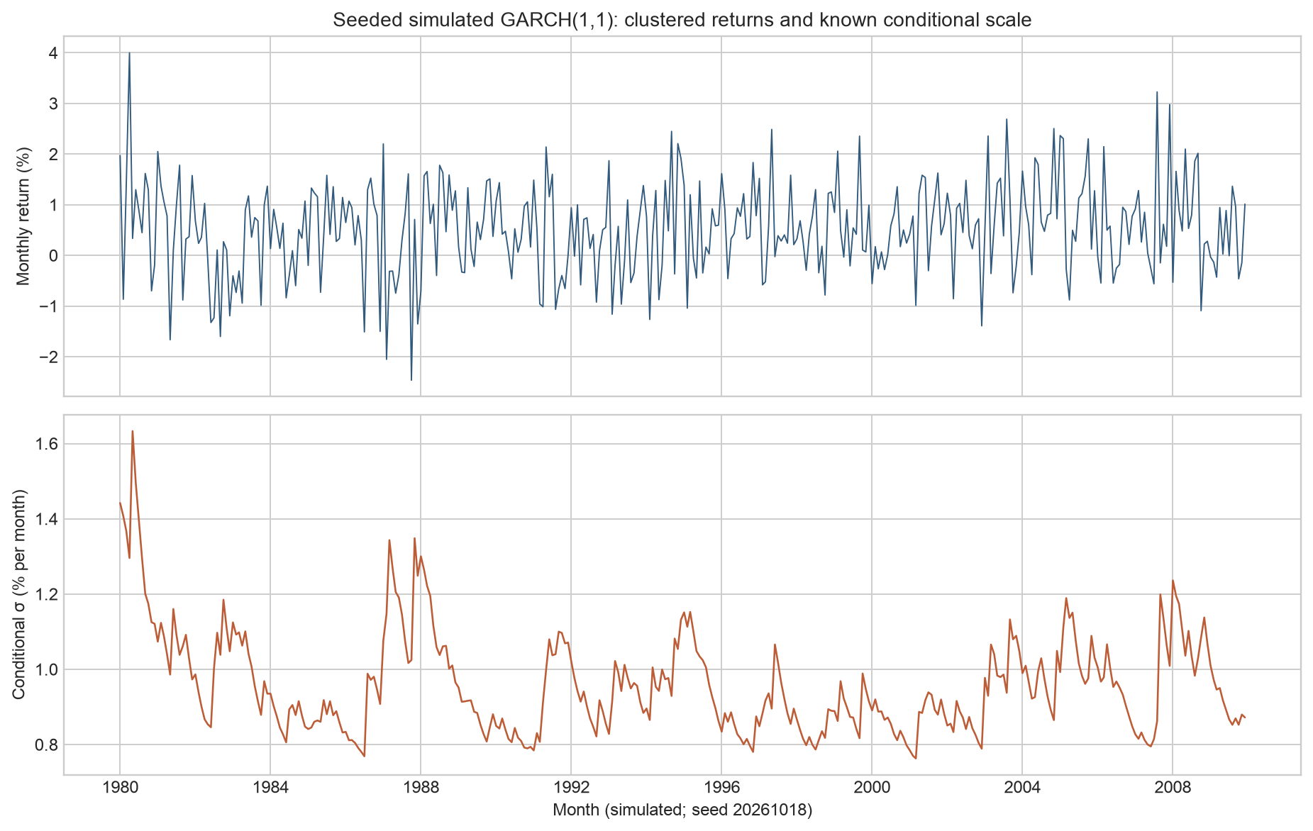
1. Simulated volatility clustering: the x-axis is simulated month (seed=20261018); the upper panel shows monthly returns in percent and the lower panel shows the true conditional standard deviation in percent/month. Larger return magnitudes cluster during high-volatility periods. The simulation’s true DGP variance is known, so it is not market evidence; finite burn-in also does not guarantee a strictly stationary initial draw.

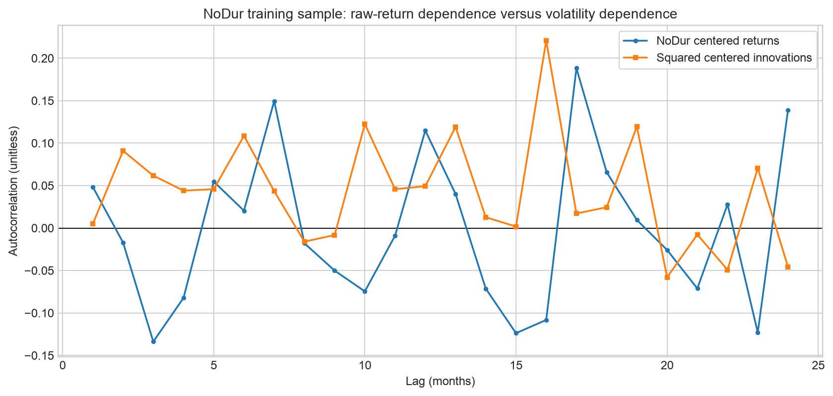
2. Return and squared-innovation autocorrelation in the real NoDur training segment: the x-axis is lag in months and the y-axis is dimensionless sample autocorrelation; the sample is the 1990–2006 training segment. Squared-innovation autocorrelations are positive at several lags, and both columns fluctuate above and below zero; the figure shows no clear, stable decay pattern. It suggests further checking for conditional heteroskedasticity, but does not establish that volatility clustering has been validated in this segment; the small-sample ACF is not a formal significance test or causal finding.

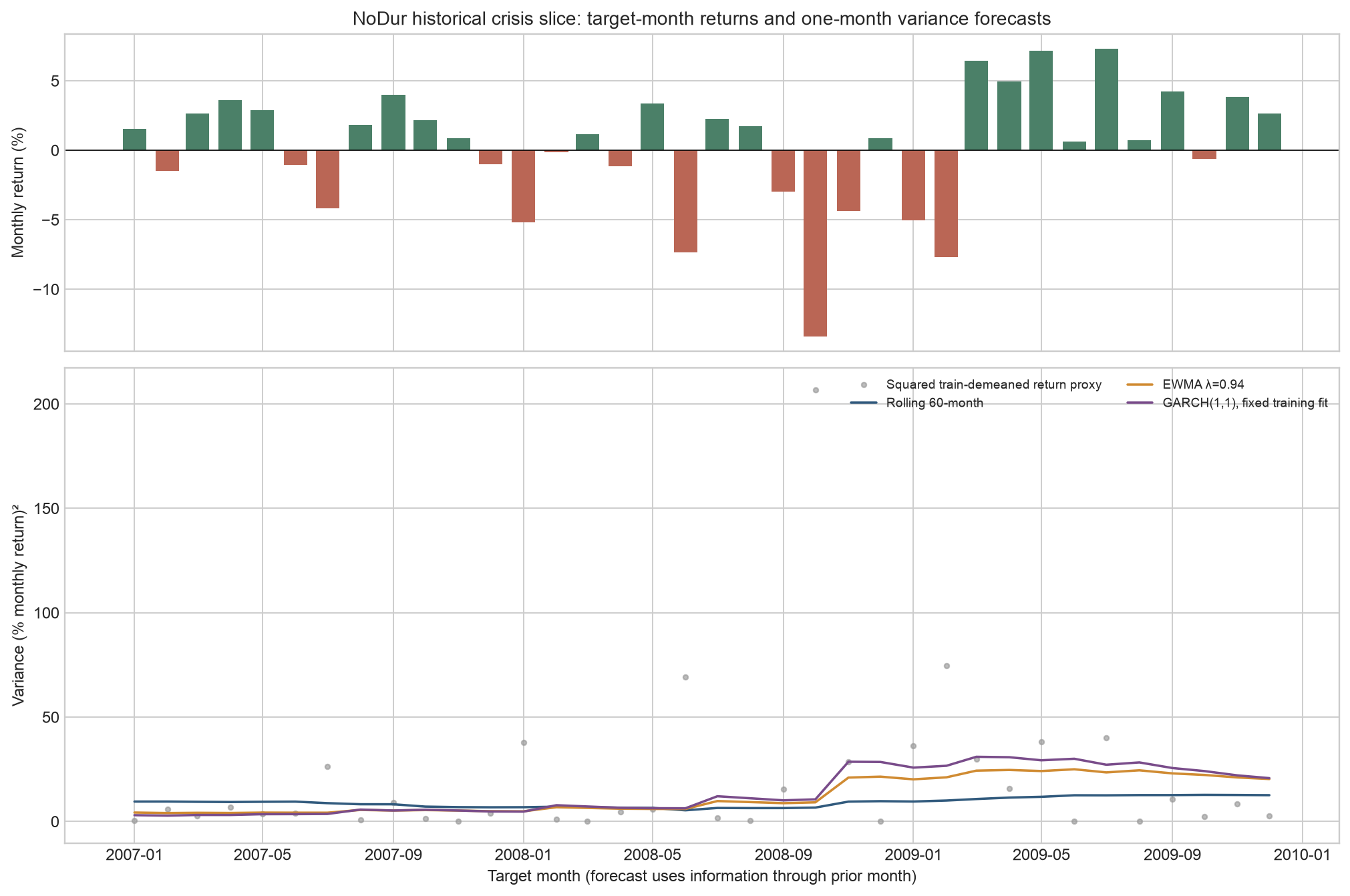
3. NoDur crisis-window forecast comparison: the x-axis is target month from 2007–2009; the upper panel shows realized monthly returns in percent and the lower panel shows $100^2\widehat h$, in “percentage monthly return squared.” Gray dots are the post hoc squared-innovation proxy; forecast curves are formed before the target month begins, and the recursion uses that month’s shock after month-end to update the next month. The historical window includes the rise in volatility in 2008, but the proxy is extremely noisy in the figure.

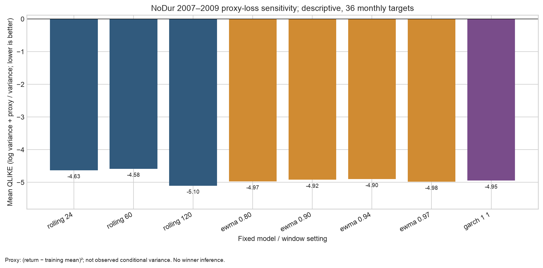
4. Proxy QLIKE sensitivity: the x-axis lists fixed model/window settings and the y-axis is average QLIKE over 36 target months; lower scores are better for the same sample and units. The caption identifies the proxy as $(r_t-\bar r_{train})^2$, not the true conditional variance. No confidence intervals, significance, or winning-model claim is provided.

11. Real-Market Example

The case uses the French Data Library’s NoDur (Consumer Non-Durables) monthly value-weighted simple returns for the 10 industry portfolios. The frozen snapshot was downloaded on 2026-10-05; the source table is in percent, and the processed table is converted to decimals by dividing by 100. It is monthly data, with return intervals defined by calendar month; the processed data end in 2026-08. NoDur is an industry portfolio rather than an individual stock. Its reported returns do not provide a transaction-cost or tradable-strategy ledger.

The research design uses 1990-01 through 2006-12 as a 204-month fitting segment and 2007-01 through 2009-12 as a 36-month historical evaluation segment specified in the script in advance. The historical crisis slice shows how the recursion behaves across a change in conditions; it is not claimed as a preregistered or independent external test. The window also cannot be selected again after seeing the result and then described as prespecified. The fixed training mean for the GARCH fit is 0.0097235, and the training-sample standard deviation is 0.0389174. The fit is:

For evaluation, use $q_t=(r_t-\bar r_{train})^2$ as the variance proxy. The mean proxy over 36 periods is 0.0019354 (decimal return squared). QLIKE results (same aligned sample and scale; lower is better) are:

Rolling 120 has the lowest proxy score here; GARCH does not have the lowest loss. All settings are retained. The sample has only 36 months, squared-return proxies may be conditionally biased, the target slice is affected by crisis conditions, and no paired forecast-loss inference was conducted; therefore, no statistical winner or future trading advantage is claimed. If the mean changes in the evaluation period, the squared deviations centered on the training mean also include mean error. The theoretical conditions for proxy-based QLIKE rankings cannot be assumed to hold as a result.

The clock boundary matters: the forecast $h_t$ uses only return shocks through (t-1); the target-month return $r_t$ can be observed only after month-end and then used for $h_{t+1}$. However, actual source-data release dates, historical revisions, and the versions visible at the time have not been archived. This is historical attribution using the current frozen snapshot, not point-in-time (PIT) or genuinely real-time out-of-sample evidence.

12. Common Mistakes

The shortest leakage demonstration is: forecast_t = eps_t**2 uses the target month’s post hoc data on the right-hand side; the correct one-step GARCH expression at the start of month $t$ is forecast_t = omega + alpha*eps_prev**2 + beta*h_prev. They are not forecasts formed at the same time.

13. Applications in Quantitative Research

A reproducible volatility study should make the following chain clear.

1. Hypothesis and target: The question here is how a one-month variance forecast behaves under historical conditions, not whether returns can be forecast in direction or what the portfolio return will be.
2. Data and version: Record the French source, download date, unit conversion, missing values, hashes, release dates, and versions. A test of what was historically available requires point-in-time data with publication times and revision versions; the current snapshot is insufficient.
3. Clock: Specify the training cutoff month, target month, signal calculation time, and time an order could be placed. A monthly return is observed only after the target month ends. The month-by-month recursion uses the previous month’s actual shock, so future values are not backfilled into earlier forecasts.
4. Benchmarks and candidates: Use rolling variance as a benchmark and compare it with fixed-parameter EWMA/GARCH; prespecify candidate settings, retain sensitivity checks, and do not pick a winner from a short evaluation period.
5. Diagnostics and loss: Check return and squared-innovation autocorrelation, conditional-standard-deviation paths, optimization boundaries, convergence counts, and units; align target months before evaluating loss. Squared innovations are not the latent true variance; QLIKE ranking has the corresponding theoretical support only under conditions such as conditional unbiasedness of the proxy.
6. External validation: Recheck across different markets, periods, frequencies, and structural changes, and report failed months and instability. If converting forecasts into positions, separately analyze actual order timing, turnover, fees, market impact, financing, borrow, and capacity.
7. Limits of the conclusion: Statistical differences in forecast loss are not differences in trading utility; without a post-cost ledger, do not calculate “net $\alpha$.” This case retains the result that Rolling 120 has lower proxy loss than GARCH; it does not repeatedly retest that result to declare a winner.

This chapter has also not run a “look-ahead in the objective” trading experiment: target-period conditional variance is a risk statistic, and no rule for placing trades using it has been defined. There is no trading ledger, so costs are “not applicable,” not “zero.” A reproducible net-$\alpha$ study would still need a signal, asset holdings, execution prices and delays, a fee schedule, borrow/financing records, capacity constraints, and a net-return series.

14. Chapter Summary

RV sums the squared increments in an already observed, finely partitioned path; conditional variance $h_t$ forecasts next-period risk using information available before the target period begins. A rolling window provides an auditable benchmark; EWMA mixes the new shock square with old variance; ARCH uses lagged shock squares; GARCH also carries forward past variance.

For a finite-second-moment GARCH(1,1) with standardized innovations of variance 1, $\alpha+\beta<1$ gives the long-run variance $\frac{\omega}{1-\alpha-\beta}$ and mean-reverting multi-step recursion; it is not the same as strict stationarity or the fourth-moment condition. EWMA’s weights sum to 1, which is precisely its boundary behavior without reversion to a separate long-run level. High-frequency RV also faces sampling and microstructure noise.

The code puts these concepts into practice through the separation of training and target data, data hashes, and the recursive clock. The historical NoDur 2007–2009 comparison shows the difference between a forecast and a squared-return proxy; it cannot establish availability at the time, a winning model, strategy profitability, or a future trading advantage.

15. Exercises

18-E01 Concept: RV and Sample Variance. In one precise sentence, compare interval RV, sample variance, and squared net return; list two path features that can make RV greater than squared net return.

18-E02 Concept: Clustering. Why can volatility clustering exist even if return autocorrelation is close to zero? Give one sample statistic to check and explain what it cannot prove.

18-E03 Concept: Stationarity and Moments. What does each of the following describe: the finite-second-moment condition, strict stationarity, and a finite fourth moment? How do they differ logically?

18-E04 Concept: EWMA. What does EWMA’s $\lambda$ control? Why does the boundary $\alpha+\beta=1$ not mean “mean reversion to some long-run variance”?

18-E05 Hand Calculation: Realized Risk. For log returns $[0.01,-0.02,0.03]$ in three subintervals of the same interval, calculate RV, RVOL, and squared net log return. Explain the units.

18-E06 Hand Calculation: EWMA. Let $\lambda=.9$, $h_1=.0004$, and the shocks be $[.01,-.02,.03]$. Write the first three monthly forecasts $h_1,h_2,h_3$ under the target convention.

18-E07 Hand Calculation: ARCH/GARCH. Let $\omega=.00001$, $\alpha=.1$, $\beta=.8$, $h_1=.0004$, and the first two shocks be .01 and $-$.02. Find GARCH $h_1,h_2,h_3$, then find ARCH $h_2,h_3$ when $\beta=0$.

18-E08 Persistence and Higher Moments. For parameters $(\omega ,\alpha ,\beta )=(.00001,.1,.8)$, calculate the long-run variance and the left-hand side of the Gaussian fourth-moment condition. Does each condition hold?

18-E09 Multi-Step Forecast. For the GARCH model above, if $h_{T+1|T}=.0004$, list the variance forecast for each target month at $k=1,2,3$. Why can’t the last number be treated as the cumulative three-month variance?

18-E10 Hand Calculation: Noise Bias. Suppose the expected sum of squared efficient-price increments over the interval is 0.001, each observation-noise variance is $\tau^2=.000001$, and the sampling count is M=10. Under the simple independent-noise model, what is the approximate expected observed RV? What about M=100?

18-E11 QLIKE. Write the average QLIKE. If proxy $q$ is conditionally unbiased and candidate variance is positive, explain why forecast risk affects expected loss; then list at least two threats to the current NoDur proxy ranking.

18-P01 Implement RV. Pass the three subinterval log returns from the same interval, $[.01,-.02,.03]$, to the shared core; assert that the result is .0014 and also display the squared net return. Explain why it is not automatically annualized.

18-P02 Forecast Clock. Use four consecutive monthly returns $[.01,.03,-.01,.02]$ and window 2; call the rolling variance forecast function (the P02 answer must include the complete code). Write the forecast for month 3, change month 3 and month 4 returns to 100, and recalculate; the month-3 forecast must remain unchanged. Explain why the first two months are NaN.

18-P03 Reproducible Research. Run the chapter CLI from any working directory and check the three input SHA-256 hashes, training and evaluation record counts, results JSON, and four figures. If a hash does not match, explain why the correct behavior is to stop rather than download the data and continue automatically.

18-C01 QML Boundary. Give three differences between core fit_garch11 and joint normal MLE; explain what “three starting points converged” can and cannot establish. List a typical set of regularity conditions for consistent QML variance estimation; do not claim it holds for arbitrary nonnormality.

18-C02 High-Frequency Microstructure. Starting from $Y_i=X_i+u_i$, derive the extra term in the expected RV from independent noise. Give one realistic assumption that may fail and design a study to test sampling frequency; do not assume one universally best frequency.

18-C03 Historical vs. PIT. Explain why the French NoDur 2007–2009 results in this chapter are neither historical PIT evidence nor a preregistered test. List the ledger fields still needed for a net strategy test, and distinguish “costs not applicable” from “costs are zero.”

18-C04 Constructed Counterexample: Strict Stationarity and Variance. For $\alpha=.1$, $\beta=.9$, and (z~ N(0,1)), compare $E(\alpha z^2+\beta )$ with $E\log(\alpha z^2+\beta )$. Explain what follows under the standard stochastic-recursion condition and what finite moment cannot be asserted.

Teaching Supplements (Independent IDs)

18-R01 Initialization Effects. Use the expansion in §5.3 for EWMA to prove that the forecast difference from two initial values decays geometrically. If the initial values differ by 0.0005 and lambda=0.9, what is the difference after two updates?

18-R02 Proxy and Unit Diagnostics. The true conditional mean is 0.01, the fixed center is 0, and the true conditional variance is 0.0004. What is the conditional expectation of the squared-return proxy? If returns are uniformly converted from decimals to percentages, by how much does QLIKE increase, and does the ranking change?

18-R03 Research Judgment. A researcher compares intraday RV with a monthly forecast and declares it unbiased because its proxy mean is close to the mean of monthly squared returns. Which conditions and records are missing?

16. Programming Exercises

Complete 18-P01–18-P03. Deliver a runnable cell or script, assertions, run command, Python and dependency environment, output paths, data version, and clock description. P02 must display the target index and NaN warmup; do not silently fill warmup rows with zeros. P03 must not touch frozen raw files or introduce a network download.

17. Challenge Problems

Complete 18-C01–18-C04. Answers may use equivalent reasoning, but must state assumptions, units, information set, and testable steps.

• For full credit on C01, distinguish the fixed training-sample mean from joint MLE; explain that consistency and robust inference are different questions; state at least three of the following: correct conditional mean/variance, stationarity and ergodicity, identification, and finite integrability; and note that the core has no parameter standard errors.
• For full credit on C02, expand the noise difference and squared expectation and propose a frequency-sensitivity plan; identify the limits of the simple derivation, including correlated noise, correlation between price changes and noise, jumps, and asynchronous observations.
• For full credit on C03, identify the missing data version/release times and historical availability, the ex post crisis slice, and the absence of position or execution ledgers; provide at least six net-return audit fields.
• For full credit on C04, use the strict Jensen inequality to distinguish $EA=1$ from $E\log A<0$; explain that a strictly stationary solution can exist while the second moment formula is infinite or does not hold; do not present the chapter’s finite-variance implementation as covering this region.

18. Complete Answers and Hints

18-E01

RV is the sum of squared log returns over subintervals within the same interval; sample variance centers on the sample mean and divides by (M-1); squared net return nets the returns first and then squares. Repeated reversals reduce the net amount, and more nonzero subintervals add to the sum of squares, so path cancellation and back-and-forth movement within an interval can both make RV greater than squared net return.

18-E02

If the signs or linear variation in innovations are unpredictable but their conditional scale changes with market conditions, then $r_t$ can have low autocorrelation while $r_t^2$ inherits persistence in the scale state. Check the sample ACF of centered squared innovations. It is a structural diagnostic; it cannot establish a causal mechanism, predict future direction, or show economic significance.

18-E03

The finite-second-moment condition $\alpha+\beta<1$ ensures a finite unconditional-variance solution in this chapter’s setup. Strict stationarity means that the joint distribution of the process does not change under time shifts; for the GARCH stochastic recursion, $E\log(\alpha z^2+\beta )<0$ is commonly used as a condition. With Gaussian shocks, a finite fourth moment additionally requires $3\alpha ^2+2\alpha \beta +\beta ^2<1$. The latter is stronger; a finite second moment suffices for the corresponding strictly stationary solution but is not necessary for strict stationarity, and strict stationarity does not ensure a second moment exists.

18-E04

$\lambda$ is the retention rate on the old variance state, and $1-\lambda$ is the weight on the latest shock square. The recursion allocates all weight between the “old forecast” and the “new shock”; it has no additional $\omega$ pulling the state toward a separate long-run level. It lies on the $\alpha+\beta=1$ boundary, so the finite-variance mean-reversion expression $\omega /(1-\alpha -\beta )$ does not apply.

18-E05

Net log return $=.02$, and squared net log return $=.0004$. RV is measured in squared decimal returns over the interval; RVOL is measured in decimal returns over the interval. There is no annualization factor.

18-E06

The third innovation, .03, generates $h_4$; it cannot affect $h_3$, which was formed before that month began.

18-E07

With $\beta=0$, $h_2=.00001+.1(.0001)=.00002$, and $h_3=.00001+.1(.0004)=.00005$. All are in squared decimal monthly returns.

18-E08

The Gaussian fourth-moment left-hand side is $3(.1)^2+2(.1)(.8)+(.8)^2=.83<1$, so both conditions hold. This result establishes a finite fourth moment only under the specified Gaussian standardized-shock and model assumptions; it cannot be generalized to arbitrary shock distributions.

18-E09

$\rho =.9,\bar h =.0001$.

These are risk forecasts for one month each. Cumulative interval variance is the sum of monthly variances only under additional conditions, including zero cross-period innovation conditional covariance given the forecast origin and a known mean; $h_{T+3|T}$ alone does not represent the three-month total.

18-E10

The variance of each noise difference is $2\tau ^2=.000002$. At M=10, the extra term is approximately .00002, so expected RV is (approximately 0.00102); at M=100, the extra term is approximately .0002, so expected RV is (approximately 0.0012). This uses a simplified independent and identically distributed noise model; it is not a frequency rule for every market.

18-E11

If $E(q_t\mid F_{t-1})=h_t^\star$, the conditional expected loss as a function of positive forecast $\widehat h$ is $\log \widehat h +h_t^\star/\widehat h$, with derivative $1/\widehat h -h_t^\star/\widehat h ^2$; it is minimized at $\widehat h$=$h_t^\star$. In the actual NoDur case, the squared proxy may be affected by differences between the training and evaluation means, high noise in a single-period square, revisions to the current data version, only 36 months of data, and date misalignment.

18-P01

Reference implementation:

from quant_course.volatility import realized_variance

parts = [0.01, -0.02, 0.03]
rv = realized_variance(parts)
net_squared = sum(parts) ** 2
assert abs(rv - 0.0014) < 1e-12
assert abs(net_squared - 0.0004) < 1e-12
print(rv, net_squared)

Output: 0.0014 0.0004. The function does not demean, divide by the sample count, or annualize; the caller must record the interval and sampling design from which these returns came.

18-P02

import pandas as pd
from quant_course.volatility import rolling_variance_forecast

idx = pd.period_range("2000-01", periods=4, freq="M")
r = pd.Series([0.01, 0.03, -0.01, 0.02], index=idx)
f = rolling_variance_forecast(r, window=2)
assert f.iloc[:2].isna().all()
assert abs(f.iloc[2] - 0.0002) < 1e-12  # sample variance of 0.01 and 0.03
r2 = r.copy(); r2.iloc[2:] = 100.0
f2 = rolling_variance_forecast(r2, window=2)
assert f2.iloc[2] == f.iloc[2]

The month-3 forecast uses only the two observations from months 1 and 2. Their sample variance is $(.01-.02)^2+(.03-.02)^2$ divided by $2-1$, which equals $.0002$. The first two target months do not have two previous observations, so they remain NaN. Changing the current or future return cannot change the month-3 forecast.

18-P03

Run from a current directory outside the repository:

cd /tmp
/absolute/path/to/quant_course/.venv/bin/python \
  /absolute/path/to/quant_course/code/ch18_volatility.py \
  --output-dir /tmp/ch18-results --figure-dir /tmp/ch18-figures

Check the JSON: train_n=204, evaluation_n=36, training endpoint 2006-12, test window 2007-01…2009-12, the three hashes match the manifest, and the paths to four figures exist. A hash mismatch means the inputs are no longer the frozen evidence for this study; silently downloading a new version would change the research object and its version. The correct action is to stop, report the difference, and establish a separate manifest for the new snapshot.

18-C01

The in-class function first computes and fixes the training-segment sample mean, then optimizes only the variance parameters; joint normal maximum likelihood optimizes the mean and variance parameters together in the same likelihood. The core objective is normalized by the scale of training residuals, omits a constant, and takes the average; after fitting, $\omega$ is multiplied back by the variance scale. Convergence from three starting points shows that at least one feasible numerical solution was found from those starts and the code selected the one with the lower objective; it does not prove a global optimum, a correct model, significant parameters, or future stability.

Typical consistency conditions can include a correctly specified (or explicitly quasi-correct) conditional mean/variance, a stationary and ergodic process, a finite and integrable objective, identified parameters with a parameter space satisfying the required conditions, and numerical optimization close to the objective’s extremum. Under nonnormality, inference usually also requires a corresponding robust variance estimate; the core provides no robust standard errors. Convergence of an in-sample fit does not replace these theoretical and empirical conditions.

18-C02

Expand $\Delta Y$, square, sum, and take expectations. The efficient-price term gives the efficient price’s squared variation; under independent, zero-mean noise, the cross-term has expectation zero; each noise difference $\Delta u$ has variance $2\tau ^2$, for an increase of approximately $2M\tau ^2$ across M intervals. Real-world noise may be serially correlated or correlated with efficient-price changes; bid–ask bounce, asynchronous trades, and jumps can also change the error structure.

First define the asset, trading hours, and target; select several sampling intervals in advance; estimate RV using the same cleaning, alignment, and interval rules, while retaining jump/noise diagnostics; compare error and robustness across dates and liquidity regimes; where possible, combine estimates of microstructure noise with alternative realized measures; and report estimation uncertainty. Do not generalize one frequency chosen in one paper for one asset to all settings.

18-C03

The data are the current French snapshot downloaded on 2026-10-05, with no historical month-by-month release versions, availability times, or local-ingestion timestamps; historical NoDur values may have been revised. The crisis slice is fixed in the script, not preregistered or an independent external test. Although the parameters are fitted before evaluation begins, the test still uses existing historical target-month returns and later recursive updates; this does not reconstruct real-time operations.

A post-cost strategy also needs: signal time, target weights/positions, executable order time, order/execution prices, spreads and fees, turnover, market impact, financing/borrow, cash/margin, capacity limits, handling of unfilled/delayed orders, and a benchmark and net-return series. Without a strategy and order ledger, costs are not applicable; this does not mean costs were set to zero or that net returns have no costs.

18-C04

Let $A=0.1z^2+0.9$. For $z\sim N(0,1)$, EA=0.1(1)+0.9=1. A is nondegenerate, and if $E|\log A|<\infty$, strict Jensen gives $E\log A<\log EA=0$. The stochastic-coefficient recursion $h_t=\omega+A_{t-1}h_{t-1}$ can therefore have a strictly stationary solution under standard conditions. However, EA=1 means the finite unconditional variance formula $\omega/(1-EA)$ does not exist, and the second moment is not finite; strict stationarity alone does not justify reporting a finite long-run h. The in-class core restricts parameters to $\alpha+\beta<1$, so it does not fit this example.

Complete Answers to the Teaching Supplements

18-R01. Subtracting the two recursions with the same shock sequence gives $\delta_{t+1}=\lambda\delta_t$, so after two updates the difference is $0.9^2\times0.0005=0.000405$. The initial value must be set before forecasting begins.

18-R02. The conditional expectation is $0.0004+(0.01-0)^2=0.0005$, giving a conditional bias of 0.0001. Uniformly converting both forecast and proxy increases the loss by log(10000), approximately 9.210340; all models on the same sample shift by the same constant, so the ranking is unchanged.

18-R03. First check whether intraday RV covers the complete target month, the return definition and units, sampling noise and jumps, whether the forecast was saved before the month, and whether the effective samples match. Unbiasedness requires the conditional expectation to match the target; close unconditional sample means do not prove conditional unbiasedness and do not establish a significant win or net return.

19. Further Reading

• Must Know — Bollerslev (1986), §§2–3. Read the GARCH representation, weak-stationarity variance condition, and GARCH(1,1) fourth-moment condition; the corresponding passages and author-PDF page references for this chapter are recorded in source_notes.md.
• Must Know — Andersen, Bollerslev, Diebold & Labys (2003), Introduction and §2. Read about the asymptotic relationship between high-frequency sums of squared returns and quadratic variation/integrated variance, including the jump term; do not misread a limit result as equality between finite-grid RV and conditional variance.
• Should Know — Hansen & Lunde (2006), Introduction, theoretical framework, empirical section and conclusion. Read how microstructure noise and frequency choice change realized-variance precision; frequency conclusions from that paper’s sample apply only to its sample and setting.
• Should Know — Patton (2011), §2 propositions and conclusion. Read the requirements for forecast-comparison losses with noisy but conditionally unbiased variance proxies; the proxy used in this chapter does not automatically meet them.
• Should Know — SciPy minimize(method="SLSQP") official documentation. Learn the constrained-optimization API, stopping precision, and solver status; stopping precision does not prove a global optimum.
• Optional — Official ARCH/GARCH forecast and EWMA API documentation. Use it to check one- and multi-step variance targets and alignment; this chapter does not install or use the arch estimator.
• Advanced — Engle (1982). The original paper is the source of ARCH, but this work checked only the bibliographic information on the author’s official page and did not obtain the full paper. You may obtain it through an institutional library and check the specific test derivation; this chapter does not cite unread passages as authority.

20. References

1. French Data Library. 10 Industry Portfolios, monthly average value-weighted returns. The original download URL is in the data manifest; the study snapshot, processing, and hashes are listed in Section 11. The table contains currently downloadable historical values, not historical point-in-time vintages.
2. Bollerslev, T. (1986). “Generalized autoregressive conditional heteroskedasticity.” Journal of Econometrics, 31(3), 307–327. DOI: 10.1016/0304-4076(86)90063-1. This chapter checks the key moment conditions against §§2–3 of the author’s original journal PDF, physical PDF pages 3–6; the specific reading range is in source_notes.md.
3. Andersen, T. G., Bollerslev, T., Diebold, F. X., & Labys, P. (2003). “Modeling and forecasting realized volatility.” Econometrica, 71(2), 579–625. DOI: 10.1111/1468-0262.00418. This chapter reads the Introduction and opening of §2; the derivation coverage is noted in the source notes.
4. Hansen, P. R., & Lunde, A. (2006). “Realized variance and market microstructure noise.” Journal of Business & Economic Statistics, 24(2), 127–161. DOI: 10.1198/073500106000000071.
5. Patton, A. J. (2011). “Volatility forecast comparison using imperfect volatility proxies.” Journal of Econometrics, 160(1), 246–256. DOI: 10.1016/j.jeconom.2010.03.034.
6. Engle, R. F. (1982). “Autoregressive conditional heteroscedasticity with estimates of the variance of United Kingdom inflation.” Econometrica, 50(4), 987–1008. DOI: 10.2307/1912773. The full paper was not obtained for this work, so no specific theorem or within-paper step is attributed to it.
7. SciPy documentation. scipy.optimize.minimize, SLSQP method. Optimizer API and stopping criterion only.
8. arch 7.2 documentation. Forecasting; EWMA variance process. Documentation consulted for definitions and alignment; the estimator was not installed or used.

Source locations, historical reading ranges, and verification limits are detailed in source_notes.md.