CHAPTER 02/ 45
Python for Quantitative Research: Getting Returns and Time Indices Right
Prerequisite: Chapter 1. After this chapter, you can rerun the same return analysis from a command line and a Notebook, explain missing values, label alignment, historical windows and execution timing, and reject unsorted or duplicate indices and nonpositive prices.
Time labels in this chapter use Coordinated Universal Time (UTC). NaN means Not a Number; we use this numerical marker for missing values. The marker alone does not explain why a value is missing.
1. Learning Objectives
By the end of the chapter, you should be able to:
- Organize a repeatable analysis using Python's built-in types, conditionals, loops, functions, type hints, imports and exceptions.
- Calculate a batch of returns with NumPy arrays, vectorization and broadcasting, and explain the meaning of every axis.
- Use pandas date indices for returns, ranking, rolling and expanding statistics, groupby, monthly resampling and missing-value checks.
- Express filters, column transformations and grouped aggregation in Polars, distinguishing eager execution from a lazy plan executed by
collect. - Read the input conditions and convergence results of SciPy numerical methods, and use Matplotlib to plot clearly identified samples with units.
- Rerun analysis in Jupyter Notebook and from the command line, record code changes in Git, and keep credentials and local data out of shared repositories.
To demonstrate these skills, obtain correct returns from one price column and explain its first missing return. Explicitly handle unsorted dates, duplicate indices and nonpositive prices. Verify that NaN remains in the output rather than becoming zero, and show that a signal forms before actual execution and the start of the holding interval, whose return is measured afterward.
2. Why Quantitative Research Needs Python
Many research errors are ordinary calculations applied to the wrong interval. An arithmetically correct ratio answers the wrong question if its endpoints come from different frequencies, assets or dates.
Python provides a common environment for reading data, numerical and statistical work, plotting and recording experiments. Define a function in a script, then call it from a Notebook to explore the data. After a fix, rerun it in a fresh process. NumPy operates on arrays; pandas operates on labeled tables. Both support batch operations, while pandas also aligns data by index labels. Labels clarify time series, but require explicit index checks.
We begin with three constructed teaching prices: 100, 110 and 99. Calculate the two interval returns by hand, then ask the libraries to reproduce each result. This checks arithmetic and time labels; it establishes neither a tradable strategy nor a real market observation.
3. Intuition
For the same asset, the first move from 100 to 110 is a gain; the second move to 99 is a loss. Adding price changes or percentages misses the fact that the second return acts on wealth after the first return. Section 8 works through the numbers.
Each observation needs an asset identity and an observation time. A price has a specified definition, such as a closing price or total-return index; a return has explicit start and end points. The fourth number in an array is insufficient without knowing its asset, time and interval.
An index labels each row. When pandas adds two Series, it pairs values by labels before calculating. A Monday/Tuesday Series plus a Tuesday/Wednesday Series leaves Monday and Wednesday missing because their partners are absent. Alignment can reveal mismatches or quietly reduce the usable sample. Check the resulting row count, missing positions and dates.
4. Mathematical Foundations
Let
Here
A one-dimensional pandas price sequence and its return output both have shape
Wealth factors multiply:
We use
For positive prices, log returns
Log and simple returns differ. Funding and ordinary portfolio weights generally use simple returns; keep the two definitions separate.
Most decimal fractions have only approximate finite binary representations. The machine result of 0.1 + 0.2 need not equal 0.3 exactly; extra trailing digits do not by themselves show a formula error. Compare floating-point results with a tolerance. Accounting that requires exact decimal amounts needs a separate decimal representation and rounding rule. Preserve price units, dtypes and tolerance conventions even when using floats for returns.
5. Definitions and Objects
Python is a general-purpose interpreted language. An expression produces a value; a statement controls execution or binds a name. A variable name binds an object and does not fix its type. Common built-in objects include int, float, bool, str, list, tuple, dict, set and None. Numeric price columns should have a defined type rather than mix dates, notes and numbers.
if/elif/else selects branches; for visits items and while repeats a check. A function names input/output logic; a module is an importable Python file or library. An exception makes failure identifiable. Type hints describe expected interfaces for readers, integrated development environments (IDEs) and static checkers. They do not automatically reject incompatible inputs at runtime.
A pandas DataFrame has row and column labels. Labels govern alignment; iloc selects by position. These rules are not interchangeable. Timestamp, DatetimeIndex and PeriodIndex can represent time points or periods.
Reading Objects and Brackets
import pandas as pd imports a module under the short name pd. A dot accesses a module function or object method; () calls it. = binds the result on the right to a name on the left; == tests equality. assert condition stops the example when the condition fails. [100, 110] is an ordered list; {"A": [100, 110]} is a dictionary mapping a string key to a value. index=dates is a named argument specifying row labels.
A Series has one column of values and an equally long Index. A DataFrame has both row and column labels. df["A"] returns a Series; df[["A"]] uses a list of column names and returns a two-dimensional DataFrame. df.iloc[1, 0] selects the second row and first column using zero-based positions. df.loc[dates[1], "A"] selects the same cell by labels. Equal positions do not prove equal labels in an imported table.
Shape mean(axis=0) removes time and returns one mean per asset; mean(axis=1) removes assets and returns one cross-sectional mean per date. rank(axis=1) ranks within each row. rolling(2).mean() moves along each column's row order and retains the date rows. Check each operation's output shape even when axis numbers coincide.
prices[1:, :] takes all rows from the second onward and all columns; prices[:-1, :] takes all but the last row. Colons slice and the comma separates row/column selections. These slices pair adjacent endpoints within a column and produce
Six Core Operations
- shift: move values a specified number of positions along an axis.
shift(1)places the previous row's value at the current time label, leaving the first value NaN. It changes alignment without changing index labels. - Rolling window: use a fixed-length historical window including the current row. For size
, the default min_periods=Wrequiresnonmissing observations; otherwise the result is NaN. - Expanding window: use all observations from the sample start through the current row. With
min_periods=1, the first row has a result and the sample grows thereafter. - groupby: partition a table by discrete keys such as
asset, calculate independently within groups, and combine the results. Grouping isolates assets but does not sort them. First sort time ascending within each group and reject duplicate keys. - resample: divide a time-indexed series into regular bins, such as weeks or months, and aggregate each bin with
.last()or.mean(). A boundary label does not assert that the market was open then. - Cross-sectional rank: rank asset characteristics or returns within a time slice along
axis=1.pct=Truenormalizes ranks to.
Polars' expression application programming interface (API) constructs column transformations. Eager mode computes each step; lazy mode first constructs a query plan for optimization and execution. SciPy supplies distributions, linear algebra, optimization, interpolation and integration on top of NumPy. Matplotlib maps numbers to graphical elements. Jupyter provides cells and a computational kernel; Git records recoverable commits.
6. Derivation
Without external cash flows, holding wealth evolves as
Expanding this recurrence gives
The prices must share a definition and refer to the same holding. Closing-price ratios understate total return when omitted dividends matter. With splits or vendor revisions, specify whether the input is raw prices, adjusted prices or a total-return series.
The denominator must be positive. Zero makes division undefined; negative prices are outside this example's ordinary spot-asset interpretation. compute_returns requires an ascending, unique, timezone-aware DatetimeIndex and positive finite nonmissing prices. It preserves and propagates NaN without filling; the caller must choose and record any cleaning rule.
7. Financial Interpretation
A return is an interval statistic. A return labeled 2026-02-28 needs explicit starting and ending times. Labels often use the interval end and cannot alone establish when a signal became available.
The course distinguishes event_time, available_at (earliest availability of that version), ingested_at (actual receipt and storage by this system), signal_time, trade_time, return_start and return_end. Eligible inputs satisfy both
Execution must follow the signal. Public but unreceived data cannot enter this system's historical signal. If equal timestamps do not establish order, exclude the version or retain finer receipt ordering; Chapter 3 explains this boundary. A signal requiring the finalized close cannot simply assume execution at that same close. An execution design must establish order submission, matching and latency. A common teaching setup forms a signal from closing information and trades at the next executable time, measuring returns after execution.
Simple returns compound over time and combine across assets using capital weights effective at the interval start, assuming no within-interval rebalancing, extra cash flows or financing. Log returns add over time but cannot replace simple returns in an ordinary capital-weighted portfolio. Keep daily, monthly and annualized quantities separate, and define annualization by frequency and market calendar. A missing trading day is not a zero return; filling zeros changes volatility, cumulative returns and correlations.
Historical rolling statistics must use information known by the signal time. A signal at close
8. Worked Numerical Examples
The following constructed teaching table uses UTC-labeled observation dates, without claiming they are verified trading sessions.
| Time index | Asset A price | Asset B price | Shape and meaning |
|---|---|---|---|
| 100.0 | 50.0 | Wide table |
|
| 110.0 | 52.0 | Asset columns Index(['A', 'B']) |
|
| 99.0 | 51.0 | One extracted Series has shape |
|
| 108.9 | 54.0 | Numeric ndarray |
8.1 Inputs, Intermediate Values and Outputs
shift and Returns
Apply P.shift(1) along rows, axis 0.
| Time | Previous A | Previous B | ||||
|---|---|---|---|---|---|---|
| 100 | NaN | NaN | 50 | NaN | NaN | |
| 110 | 100 | 52 | 50 | |||
| 99 | 110 | 51 | 52 | |||
| 108.9 | 99 | 54 | 51 |
At
Rolling Mean, window=2
For A's input rolling(window=2).mean() gives:
| Time | Window | Calculation | Output |
|---|---|---|---|
| NaN | |||
| 105 | |||
| 104.5 | |||
| 103.95 |
Expanding Mean, min_periods=1
The same A input under expanding(min_periods=1).mean() gives:
| Time | Accumulated window | Calculation | Output |
|---|---|---|---|
| 100 | |||
| 105 | |||
| 103 | |||
| 104.475 |
Rolling retains a fixed lookback; expanding keeps accumulating all history.
groupby in Long Format
Flattening the full table gives eight rows with asset, date and price. A global df['price'].shift(1) can pair different assets: when rows alternate by date, the preceding row may belong to another security; with asset blocks, B's first row may use A's last price. df.groupby('asset')['price'].shift(1) shifts separately and leaves each asset's first value NaN.
For the first two dates, sorted by date and asset:
| Row | date/asset/price | Global previous | Within-asset previous | Correct return |
|---|---|---|---|---|
| 0 | t0/A/100 | NaN | NaN | NaN |
| 1 | t0/B/50 | 100 (A) | NaN | NaN |
| 2 | t1/A/110 | 50 (B) | 100 (A) | 0.10 |
| 3 | t1/B/52 | 110 (A) | 50 (B) | 0.04 |
The global calculation produces
resample
.resample('W-FRI').last() assigns observations from Monday January 5 through Thursday January 8 to the bin ending Friday January 9. The output label is 2026-01-09, but A's value 108.9 comes from January 8, the last input observation. A bin boundary does not establish a trading session.
Cross-sectional Percentile rank
At returns.rank(axis=1,pct=True) compares assets on that date: B has rank 1 and percentile
Axis checks on prices give P.mean(axis=0) = A 104.475, B 51.75, shape P.mean(axis=1) = 75, 81, 75, 81.45, shape
Label alignment gives January 5: shift(1) retains January 5–8 labels and changes A's values to NaN/100/110/99. shift(1,freq="D") retains 100/110/99/108.9 and moves labels to January 6–9. Neither establishes executable prices.
With average ranks, two equal 1% returns have rank 1.5 each and percentile
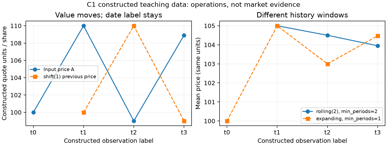
The horizontal axis contains constructed
8.2 Three Price Observations, Two Compounding Intervals
8.3 Compatible Shapes Can Still Use the Wrong Axis
A shape
Here
To scale risky capital by date, use a column vector
Row sums are −2% and 3%. In the second interval the asset weights are 0.10/0.40 and cash is 0.50; the budget remains 1.
The wrong
This halves B in both intervals instead of halving risky exposure only in the second. Multiplying by g[:,None] explicitly retains the time axis with shape
import numpy as np
r = np.array([[0.10, -0.05], [-0.10, 0.10]])
w = np.array([0.20, 0.80])
g = np.array([1.00, 0.50])
asset_contributions = r * w
date_contributions = (r * g[:, None]) * w
wrong_contributions = (r * g) * w
assert np.allclose(asset_contributions.sum(axis=1), [-0.02, 0.06])
assert np.allclose(date_contributions.sum(axis=1), [-0.02, 0.03])
assert np.allclose(wrong_contributions.sum(axis=1), [0.00, 0.02])
9. Python Implementation
Default Entry in the Accepted Reader Package
This sample carries forward the shared implementation of the accepted I3 reader. Create the environment following the reader installation instructions, then run from the reader-package root:
.venv/bin/python run_notebook.py notebooks/ch02_python.ipynb
The default Notebook uses packaged shared logic, reads no absent French data and downloads nothing. New outputs go to a unique runs subdirectory. The course-root code, lock file and historical tests below are the original working-source route; do not mix the two roots. Optional French files require authorized inputs under the optional-data contract and were not rerun for this batch. The reader CLI uses a new UUID directory and rejects overwrites. Constructed runs do not validate market data or fills.
Begin with ordinary expressions and list indexing:
prices = [100.0, 110.0, 99.0]
first_return = prices[1] / prices[0] - 1.0
second_return = prices[2] / prices[1] - 1.0
wealth = 100.0 * (1.0 + first_return) * (1.0 + second_return)
assert abs(wealth - 99.0) < 1e-12
print(first_return, second_return, wealth)
A caller supplies function inputs; the body calculates; return gives the result back. This standalone example demonstrates hints and explicit failure boundaries:
from collections.abc import Sequence
from math import isfinite
from numbers import Real


def final_wealth(initial: float, returns: Sequence[float]) -> float:
    if isinstance(initial, bool) or not isinstance(initial, Real):
        raise TypeError("initial must be a real number")
    if not isfinite(initial) or initial <= 0.0:
        raise ValueError("initial must be positive and finite")
    wealth = initial
    for value in returns:
        if isinstance(value, bool) or not isinstance(value, Real):
            raise TypeError("returns must be real numbers")
        if not isfinite(value) or value < -1.0:
            raise ValueError("simple return must be finite and at least -100%")
        wealth *= 1.0 + value
        if not isfinite(wealth):
            raise ValueError("wealth exceeds finite numeric range")
    return wealth


assert abs(final_wealth(100.0, [0.10, -0.10]) - 99.0) < 1e-12
for invalid in ([float("nan")], [float("inf")], [-1.01], [True], ["0.1"]):
    try:
        final_wealth(100.0, invalid)
    except (TypeError, ValueError):
        pass
    else:
        raise AssertionError("invalid return was accepted")
print(final_wealth(100.0, [0.10, -0.10]))
This teaching function rejects non-real inputs, booleans, NaN, infinity and returns below −100%, and checks compounding overflow. The research vector interface still uses Chapter 11's wealth_index rather than a second implementation. Allowing −100% to reduce wealth to zero does not establish defined account returns after bankruptcy. Type hints help tools but do not enforce inputs. ValueError rejects known contract violations. Catch only exception types you can handle; except Exception: pass hides data problems.
Imports bind reusable modules, commonly import numpy as np and import pandas as pd, or one imported function. Avoid local files called pandas.py, scipy.py or statistics.py that may shadow the intended module. An entry under if __name__ == "__main__": lets a script run directly and also be imported by a Notebook.
An isolated environment reduces dependency conflicts. The course interpreter and dependency versions are locked in Environment setup. From the course root:
python3 -m venv .venv
.venv/bin/python -m pip install -r requirements-a1-lock.txt
.venv/bin/python -m pip install -e . --no-deps
.venv/bin/python -m pytest tests -q
.venv/bin/python tools/run_a1.py
The lock file identifies the course snapshot. Temporary package exploration can use a disposable environment, but formal results return to the project environment and run from the beginning. Command-line and Notebook entry points share .venv; select its Python kernel. The src layout and editable installation make both import the same core functions.
The API is compute_returns(prices: pd.Series, kind: Literal["simple", "log"] = "simple") -> pd.Series, imported with from quant_course import compute_returns. The price index must be ascending, unique and timezone-aware; nonmissing prices must be positive and finite. A missing current price makes its return missing and also makes the following return missing because that row lacks a predecessor. The first result is NaN; nothing is filled. Check inputs and outputs explicitly. When passing this series to Chapter 11's wealth_index, exclude only the first position with no preceding price; all remaining holding intervals must be complete simple returns, with initial capital supplied separately. dropna() cannot erase unknown interior intervals and preserve a continuous path. Chapter 11 §9 provides the runnable bridge; that chapter remains a Chinese prerequisite until its later translation.
From the course root, run the script or start a Notebook:
.venv/bin/python code/ch02_python.py
.venv/bin/jupyter lab
The script locates the course root from its own path and adds src to the import path. The Notebook searches upward from its working directory. Both call the same return function.
Git records which code an analysis used. In an initialized course repository, inspect status, stage explicit files, inspect the staged diff, then commit:
git status
git add code/ch02_python.py notebooks/ch02_python.ipynb
git diff --staged
git commit -m "Add Chapter 2 Python examples"
git log --oneline -1
The staging area selects changes for the next commit. A commit is local; pushing is a separate action. Exclude environments, caches and local secrets:
.venv/
.env
*.ipynb_checkpoints/
Keep API keys, passwords and access tokens out of scripts, Notebook outputs and commits. Inject them through environment variables or managed credentials, and redact run records. .gitignore only prevents untracked files entering new commits. If a secret was committed, revoke and rotate it; later deleting the file does not resolve the exposure.
NumPy applies one expression to an array. In this separate three-row example, rows are dates and columns are assets; a length-
import numpy as np

prices = np.array([[100.0, 200.0], [110.0, 190.0], [99.0, 209.0]])
returns = prices[1:, :] / prices[:-1, :] - 1.0
weights = np.array([0.5, 0.5])
weighted_asset_returns = returns * weights
portfolio_returns = weighted_asset_returns.sum(axis=1)
assert prices.shape == (3, 2)
assert returns.shape == (2, 2)
assert np.allclose(portfolio_returns, [0.025, 0.0])
print(returns, portfolio_returns)
Shape compatibility does not establish that asset columns and weights are in the same order. Label and align weights before treating the result as a portfolio.
pandas aligns Series by index labels rather than row positions. This example produces three date labels, with NaN where the other side has no partner:
import pandas as pd

dates = pd.to_datetime(["2026-01-05", "2026-01-06", "2026-01-07"], utc=True)
left = pd.Series([0.01, 0.02], index=dates[:2], name="left")
right = pd.Series([0.03, 0.04], index=dates[1:], name="right")
combined = left + right
assert abs(combined.loc[dates[1]] - 0.05) < 1e-12
assert pd.isna(combined.loc[dates[0]])
assert pd.isna(combined.loc[dates[2]])
print(combined)
Executable Small-Table Operations
The following self-contained code reproduces all six operations in §8—shift, rolling, expanding, groupby, resample and rank—and asserts their values and intermediate behavior.
from math import isclose
import pandas as pd

dates = pd.to_datetime(["2026-01-05", "2026-01-06", "2026-01-07", "2026-01-08"], utc=True)
df_small = pd.DataFrame(
    {"A": [100.0, 110.0, 99.0, 108.9], "B": [50.0, 52.0, 51.0, 54.0]},
    index=dates,
)

# 1. shift and returns
df_shifted = df_small.shift(1)
df_returns = df_small / df_shifted - 1.0
assert pd.isna(df_shifted.iloc[0, 0])
assert isclose(df_returns.loc[dates[1], "A"], 0.10, rel_tol=1e-12)
assert isclose(df_returns.loc[dates[2], "A"], -0.10, rel_tol=1e-12)

# 2. rolling(2)
rolling_mean = df_small.rolling(window=2).mean()
assert pd.isna(rolling_mean.iloc[0, 0])
assert rolling_mean.loc[dates[1], "A"] == 105.0
assert rolling_mean.loc[dates[2], "A"] == 104.5

# 3. expanding(1)
expanding_mean = df_small.expanding(min_periods=1).mean()
assert expanding_mean.loc[dates[0], "A"] == 100.0
assert expanding_mean.loc[dates[1], "A"] == 105.0
assert isclose(expanding_mean.loc[dates[2], "A"], 103.0)

# 4. Cross-sectional rank(axis=1)
ranks = df_returns.rank(axis=1, pct=True)
assert ranks.loc[dates[1], "B"] == 0.5
assert ranks.loc[dates[1], "A"] == 1.0

# 5. Long-table groupby shift
df_long = (
    df_small.reset_index()
    .melt(id_vars="index", var_name="asset", value_name="price")
    .rename(columns={"index": "date"})
    .sort_values(["asset", "date"])
    .reset_index(drop=True)
)
df_long["prev_price"] = df_long.groupby("asset")["price"].shift(1)
df_long["ret"] = df_long["price"] / df_long["prev_price"] - 1.0
assert pd.isna(df_long.loc[0, "ret"])  # First row of A
assert pd.isna(df_long.loc[4, "ret"])  # First row of B
assert isclose(df_long.loc[1, "ret"], 0.10, rel_tol=1e-12)
assert isclose(df_long.loc[5, "ret"], 0.04, rel_tol=1e-12)

# 6. Weekly resample aggregation
weekly_last = df_small.resample("W-FRI").last()
assert weekly_last.index[0] == pd.Timestamp("2026-01-09", tz="UTC")
assert weekly_last.loc[pd.Timestamp("2026-01-09", tz="UTC"), "A"] == 108.9
Polars eager operations immediately return a DataFrame. Lazy operations build a plan and execute at collect. Filtering and selecting columns let the optimizer attempt to reduce file reading:
import polars as pl

data = pl.DataFrame(
    {
        "asset": ["A", "A", "B"],
        "date": [1, 2, 2],
        "return": [0.01, 0.02, -0.01],
    }
)
eager_result = (
    data.filter(pl.col("date") >= 2)
    .group_by("asset")
    .agg(pl.col("return").mean().alias("mean_return"))
)
lazy_query = (
    data.lazy()
    .filter(pl.col("date") >= 2)
    .select("asset", "return")
    .group_by("asset")
    .agg(pl.col("return").mean().alias("mean_return"))
)
print(lazy_query.explain())
lazy_result = lazy_query.collect()
assert lazy_result.height == eager_result.height
print(lazy_result)
Optimization depends on the actual plan and source. Check schema, missingness and sorting yourself; grouped results need not retain input order.
SciPy convergence cannot establish financial assumptions. Suppose 100 currency units are received in two years and have present value 90. Under annual compounding, solve for the unknown annual rate:
from scipy.optimize import brentq


def pricing_error(rate: float) -> float:
    return 100.0 / (1.0 + rate) ** 2 - 90.0

rate = brentq(pricing_error, 0.0, 1.0)
assert abs(pricing_error(rate)) < 1e-10
print(rate)
brentq requires opposite signs at the bracket endpoints. This example assumes specified cash-flow timing, annual compounding and no default. Actual security yields also depend on day count, calendars, cash flows, clean/dirty prices and call provisions. A root finder does not define a yield.
10. Visualization
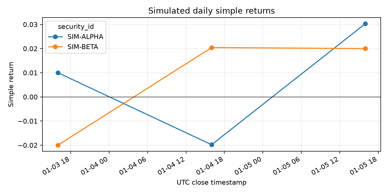
This inherited figure uses two constructed securities, SIM-ALPHA and SIM-BETA. Its horizontal axis is UTC closing timestamps; its vertical axis is dimensionless simple-return decimals. The first missing return is not connected or drawn as zero. The title says simulated and the source is a local fixture. It is neither market observation nor a plot of §8's hand example.
A caption must identify simulated data, daily observations and UTC closing labels. A Figure is the whole image and an Axes is one plotting area. Set axis labels, units, legend, title and source before saving. A reader should understand the plot from the caption alone. A real French monthly plot would need its own version, frequency and return units.
11. Real Market Example: An Inherited Snapshot
Kenneth R. French Data Library publishes research-portfolio returns at monthly or daily frequencies. This chapter's snapshot selects the Average Value Weighted Returns -- Monthly block of 10 Industry Portfolios. The inherited official description covers July 1926 through August 2026; the local processed file contains 1,202 months and ten industry columns. The original YYYYMM rows contain percentages. Processing divided them by 100 and retained YYYYMM month strings. Annual and equal-weighted blocks in the same source file must not enter this monthly value-weighted series. Daily returns come from a separate official file.
The processed monthly industry CSV has a data manifest. Download time: 2026-10-05 19:18:24 UTC. ZIP SHA-256: ebd937a4b995d821867aeb956a96f09a666386f38fa82516b7d1767ee4a49ae5. Processed SHA-256: 3b097d810c295d64eedfa1ece7067ff2a0707f5ca90e33935df9949251f70950. Historical returns can change with CRSP revisions; preserve snapshot, download date and hashes. Fama and French retain copyright. Public download does not imply unrestricted redistribution; check terms before releasing derived data.
The monthly block begins near line 12 of the original file. Missing codes are −99.99 and −999. Processing selects that block, maps those codes to NaN, constructs a monthly PeriodIndex from YYYYMM and divides percentages by 100. The manifest records compressed, extracted and processed hashes. In the first month, 192607, NoDur is 0.0144 and Durbl is 0.1558.
Read the processed file and convert its month index:
import pandas as pd

raw = pd.read_csv(
    "data/processed/french_10_industries_monthly.csv",
    dtype={"month": "string"},
)
month = pd.PeriodIndex(raw.pop("month"), freq="M")
monthly_returns = raw.set_axis(month, axis="index")
assert abs(monthly_returns.loc[pd.Period("1926-07", freq="M"), "NoDur"] - 0.0144) < 1e-12
assert abs(monthly_returns.loc[pd.Period("1926-07", freq="M"), "Durbl"] - 0.1558) < 1e-12
print(monthly_returns.index.min(), monthly_returns.index.max())
These are portfolio returns, not daily OHLCV bars. They support exercises on frequency alignment, indices, ranking and grouping; they provide neither individual daily stock prices nor company-filing availability, historical constituents or delisting records. Do not present monthly portfolio returns as prices or future-investable decision times. This section describes format and reading rules, without claims about prediction, excess return or strategy performance.
12. Common Mistakes
Adding percentages. For 100, 110, 99,
Using shift(-1) as an available feature. It moves future values to current labels. This may construct a research target, but not a contemporaneously known input. Draw a timeline and check all inputs against signal_time.
Shifting a long panel globally. Alternating assets can pair A with B's price. Sort within asset groups and shift there, or use a checked date-by-asset wide table.
Ignoring alignment. Assigning a differently indexed Series to a DataFrame matches labels, not positions. Verify equal indices or reindex explicitly. Positional assignment requires proof of equal row order.
Misaligning rolling signals and future returns. returns.rolling(20).mean() includes the current row and retains its label. A close-signal.shift(1) * returns is a teaching row alignment; actual research still needs executable interval endpoints.
Creating observations at calendar month-end. .resample("ME").last() labels a monthly bin but uses its last available input. Assets may have different actual dates, and the boundary may be a nontrading day. Analyze monthly returns as returns; do not apply a price ratio again.
Treating missing as zero. A first endpoint, vendor omission, suspension or absence of trades does not establish zero return. compute_returns preserves NaN; cleaning and selection must be explicit. Filling zero before compounding invents a return.
Chained assignment. Under pandas 3.0 Copy-on-Write, df["ret"][mask] = 0 does not modify the original object. Use df.loc[mask, "ret"] = 0 and verify the result.
Calling decimal changes percentages. A pandas ratio of 0.01 means 1%, not 0.01%. Convert for a percent-labeled plot while retaining decimals for calculations.
Trusting an already-run Notebook. Cells can run out of order and retain stale variables. Save, restart the kernel and run all cells top to bottom. Rerun scripts in fresh processes and record library versions, input paths and parameters.
13. A Research Workflow
Start by defining assets and data: IDs, price convention, currency, frequency, source and version. Preserve raw data or a verifiable snapshot. Check time coverage, duplicate labels, sorting, dtypes, units and missingness after reading. Keep timezone information and use the market calendar to define sessions.
Use the shared return function. Start with §8's hand inputs, then verify contract failures for unsorted/duplicate dates and zero/negative prices. A missing interior price must leave its own and the next return missing. If downstream calculations need completeness, the caller explicitly selects the sample and records omissions. Automatic sorting or zero filling must not hide failures.
Define signals next. For cross-sectional ranks, establish which assets have available values on each date. Rank rows in a wide table, or group a long table by time before ranking assets. Compute historical windows within assets; shift prices and returns within the same asset. Record signal_time and each holding interval's trade_time, return_start and return_end.
Align signals to realizable subsequent returns, deduct interpretable trading and financing costs, and compare a simple benchmark. Report dates, valid counts, missingness rules, annualization, turnover and parameters. Select windows in training, assess decisions in validation and reserve testing for final evaluation. Save scripts, Notebooks, environment, configuration, figures and manifests. Report outcomes that fail the prespecified direction; a cumulative-return chart alone cannot show causation or lasting advantage.
A benchmark may equally weight the same universe or use a defined passive portfolio. Falsifying outcomes include benchmark-like returns, disappearance after costs, reliance on future data or one short period, and direction changes under small parameter variations. Python makes computations repeatable; evidence must still support the hypothesis.
14. Chapter Summary
Code defines operations; labels define their assets and times. NumPy broadcasts by shape, pandas aligns by labels, and Polars lazy API defers a plan. None chooses an appropriate financial definition for you.
Check positive prices, order, unique indices, frequency and missingness. Label returns by defined intervals, form signals from available inputs and align them to executable later holdings. Compound simple returns; use only signal-time information in windows. The command line, Notebook, plots and Git record should identify the same code, environment, snapshot and parameters.
15. Exercises
Complete answers are in §18. The first seven require no new package installation.
2-E01 — Concepts. Do Python type hints automatically validate arguments at runtime? Give an input check you would place in a financial function.
2-E02 — Concepts. An array has shape (5,3), with asset columns. How does a (3,) weight vector broadcast? How would you verify column meanings and weight order?
2-E03 — Concepts. How does pandas pair observations when adding Series with different date indices? Give a cause of alignment-induced NaN.
2-E04 — Concepts. Compare shift(1) and shift(1,freq="D"). Which moves values and which changes labels?
2-E05 — Hand Calculation. Prices move 80 → 100 → 90. Calculate both simple returns, cumulative simple return and summed price changes. Explain the differences.
2-E06 — Hand Calculation.
2-E07 — Hand Calculation. A month's trading-day closing prices are 20, 21, 19; the first next-month price is 20. What is this month's closing observation and return? Why not invent a nontrading month-end observation at 19?
2-N01 — Identify the Mechanism.
- Explain axis=0 and axis=1. Which computes each asset's time-series 20-observation mean and which ranks assets on a date?
- Why must the first shift-based return be NaN? What fictional assumption does fillna(0) introduce?
- Compare the historical information retained by rolling(window=3) and expanding(min_periods=1).
2-N02 — One Operation at a Time. For four consecutive trading-day prices
2-N03 — Complete Calculation. Use §8's A/B wide table. Calculate both assets'
2-B01 — Broadcasting Axes. For §8.3, calculate every cell after asset weighting, proper date scaling and mistaken column scaling by the one-dimensional date vector. Compare the three portfolio sequences. Explain second-period cash, g[:,None]'s shape and why length checks fail when T=N.
16. Programming Exercises
2-P01 — Returns and Failure Conditions. Call compute_returns on UTC-indexed [100,110,99]; check simple returns, the first NaN and cumulative result. Assert failures for unsorted and duplicate indices, zero and negative prices. With an interior NaN, assert missing-value propagation and show that a completeness check rejects silent zero filling.
2-P02 — Multiple Assets. Construct a shuffled long table with at least two assets and six dates. Sort, shift within assets, calculate returns, three-interval rolling return means and datewise cross-sectional ranks. Assert missing first returns, no A/B predecessor contamination and prediction inputs restricted to the current or earlier date.
2-P03 — Month-end and French Format. From the course root, read the processed snapshot. Build a YYYYMM PeriodIndex without dividing its decimal returns by 100 again. Assert July 1926 NoDur=0.0144 and Durbl=0.1558; display coverage and missing counts. Use three constructed business-day prices to show that monthly .last() selects the last input observation; do not recalculate returns from monthly returns.
2-N04 — Diagnose Code. An intern uses this panel feature code:
# Long-table feature code to diagnose
import pandas as pd
df = pd.DataFrame({
    'asset': ['B', 'A', 'B', 'A', 'B', 'A'],
    'date': ['2026-01-02', '2026-01-01', '2026-01-01', '2026-01-03', '2026-01-03', '2026-01-02'],
    'price': [52.0, 100.0, 50.0, 99.0, 51.0, 110.0]
})
# The intern shifts globally and fills zero
df['lag_price'] = df['price'].shift(1).fillna(0.0)
df['return'] = (df['price'] - df['lag_price']) / df['lag_price']
Identify the unsorted cross-asset mismatch and zero denominators/fictitious returns. Supply self-contained corrected code and assert within-group isolation.
17. Challenge Problems
2-C01 — Executable Signal Design. Design a monthly cross-sectional signal ranking the preceding 20 observed returns. Specify availability, signal_time, trade_time, return_start and return_end; map closing inputs to subsequent execution. Handle suspensions, missing returns, nontrading month-ends and rank ties. Extra prerequisites: calendars and portfolio weights. Ten points: timing contract 4, missingness/ties 2, interval calculations 2, costs/benchmark 2.
2-C02 — Memory and Query Plans. For T=1,000,000 and N=500, estimate float64 price-matrix bytes and the cost of an additional equally shaped difference matrix. Write a Polars lazy query filtering dates, selecting needed columns, deriving a column and aggregating by asset. Explain predicate/projection pushdown. Extra prerequisites: array bytes, schema and lazy plans. Ten points: memory 3, lazy/collect 3, optimization 2, memory/sorting limits 2.
2-N05 — Research Judgment. A report uses df['price'].resample('ME').last() for monthly rebalancing and claims to obtain monthly returns and immediately trade at each calendar month-end close. Diagnose:
- Calendar boundaries versus real trading days.
- The ordering problem in a zero-latency same-close fill.
- Stale .last() prices for stocks suspended several days before month-end.
18. Complete Solutions
2-E01. Hints describe expected types to static tools; the interpreter does not enforce them. Explicitly check ascending/unique indices and finite positive prices, raising ValueError for violations. Inspect NaN separately; hints do not replace runtime checks.
2-E02. The three entries match columns and repeat across rows. Verify column labels/order, reindex labeled weights to prices.columns and reject missing weights. Assert the column count equals weight length and label sets agree.
2-E03. pandas pairs index labels. A/B on the left and B/C on the right produce A/B/C; A and C lack partners and become NaN. Equal row numbers are insufficient.
2-E04. shift(1) retains the index and maps the preceding value to the current label. shift(1,freq="D") retains values/order and moves labels one calendar day forward. A previous trading observation need not be yesterday.
2-E05. Returns are
2-E06. At
2-E07. The last input is 19, so the monthly closing observation is 19. The preceding month's closing price is absent, so a full-month return cannot be calculated. From this month's first observation 20 to 19, the narrower interval returns −5%. A nontrading day has no new close; do not invent or repeat an observation.
2-N01.
- axis=0 aggregates across rows/time; use it for asset time-series means. axis=1 works across columns/assets within a timestamp; use it for cross-sectional ranks.
- The first row lacks
. Filling zero invents an observed zero-return interval and changes the valid count from T−1 to T, affecting mean and volatility. Multiplication by 1 does not change ending wealth but cannot turn an endpoint into an observed holding interval. - Rolling retains only the latest fixed
observations and forgets older ones, suited to local changing statistics. Expanding keeps all available history from the start and grows without forgetting.
2-N02. The shifted sequence is
2-N03. Returns to four decimals:
| Time | A | B | A percentile | B percentile |
|---|---|---|---|---|
| NaN | NaN | NaN | NaN | |
| 1.0 | 0.5 | |||
| 0.5 | 1.0 | |||
| 1.0 | 0.5 |
Sort the long table by asset/date and compute unfilled ratios inside groups, or pct_change(fill_method=None). A yields [0.10,−0.10,0.10], B yields [0.04,−0.0192,0.0588] and both begin NaN, exactly matching their wide columns before rounding.
2-B01. Baseline contributions are (0.02,−0.04)/(−0.02,0.08), with −2%/6% returns. Correct date-scaled contributions are (0.02,−0.04)/(−0.01,0.04), with −2%/3%. Wrong column scaling gives (0.02,−0.02)/(−0.02,0.04), with 0%/2%. Correct second-period risky weights are 0.10/0.40 and cash is 0.50. g[:,None] is (2,1), explicitly indexed by date; a one-dimensional (2,) vector aligns to the last dimension. Equal lengths cannot prove semantic alignment.
2-P01 — Reference Implementation. Run from the course root using the shared API:
import pandas as pd
from quant_course import compute_returns

dates = pd.date_range("2026-01-02", periods=3, freq="B", tz="UTC")
prices = pd.Series([100.0, 110.0, 99.0], index=dates, name="price")
got = compute_returns(prices, kind="simple")
assert pd.isna(got.iloc[0])
assert abs(got.iloc[1] - 0.10) < 1e-12
assert abs(got.iloc[2] + 0.10) < 1e-12
assert abs((1.0 + got.iloc[1]) * (1.0 + got.iloc[2]) - 0.99) < 1e-12

def must_raise_value_error(bad):
    try:
        compute_returns(bad, kind="simple")
    except ValueError:
        return
    raise AssertionError("invalid index or price was accepted")

must_raise_value_error(prices.iloc[::-1])
duplicated = pd.Series([100.0, 110.0], index=[dates[0], dates[0]])
must_raise_value_error(duplicated)
must_raise_value_error(pd.Series([100.0, 0.0], index=dates[:2]))
must_raise_value_error(pd.Series([100.0, -1.0], index=dates[:2]))

with_missing = pd.Series([100.0, float("nan"), 99.0], index=dates)
missing_returns = compute_returns(with_missing, kind="simple")
expected_valid = with_missing.notna() & with_missing.shift(1).notna()
expected_valid.iloc[0] = False
assert missing_returns.notna().equals(expected_valid)
silently_filled = missing_returns.fillna(0.0)
assert not silently_filled.notna().equals(expected_valid)
Valid returns are 0.10 and −0.10, cumulative −0.01. An interior missing price removes its current return and the following return. The last lines show why absence of NaN after filling is dangerous; actual research must record selection and missingness rather than use this fill in results.
2-P02 — Reference Implementation. This constructed six-date table ensures at least one valid three-return rolling mean and lagged signal.
import pandas as pd

rows = [
    ("A", "2026-01-06", 104.0), ("B", "2026-01-01", 50.0),
    ("A", "2026-01-01", 100.0), ("B", "2026-01-06", 58.0),
    ("A", "2026-01-02", 101.0), ("B", "2026-01-02", 52.0),
    ("A", "2026-01-03", 103.0), ("B", "2026-01-03", 53.0),
    ("A", "2026-01-05", 105.0), ("B", "2026-01-05", 55.0),
    ("A", "2026-01-04", 102.0), ("B", "2026-01-04", 54.0),
]
df = pd.DataFrame(rows, columns=["asset", "date", "price"])
df["date"] = pd.to_datetime(df["date"], utc=True)
df = df.sort_values(["asset", "date"]).reset_index(drop=True)

df["previous_price"] = df.groupby("asset", sort=False)["price"].shift(1)
df["return"] = df["price"] / df["previous_price"] - 1.0
df["mean_3"] = (
    df.groupby("asset", sort=False)["return"]
    .rolling(window=3, min_periods=3)
    .mean()
    .reset_index(level=0, drop=True)
)
df["signal"] = df.groupby("asset", sort=False)["mean_3"].shift(1)

cross_section = df.pivot(index="date", columns="asset", values="return")
rank = cross_section.rank(axis=1, pct=True, method="average")
assert df.groupby("asset").head(1)["return"].isna().all()
a = df.loc[df["asset"].eq("A")].reset_index(drop=True)
b = df.loc[df["asset"].eq("B")].reset_index(drop=True)
assert a.loc[1, "previous_price"] == 100.0
assert b.loc[1, "previous_price"] == 50.0
assert df.groupby("asset")["signal"].apply(lambda s: s.notna().any()).all()
print(df)
print(rank)
Sort before shifting within each group. The rolling window requires three valid returns; the initial rows do not yet provide them. Shift the mean again so a same-row estimate is not applied to that row's return interval. rank compares assets at one date, without mixing A's multiple dates into B's cross-section.
2-P03 — Reference Implementation. The processed returns are already decimals.
from pathlib import Path
import pandas as pd

path = Path("data/processed/french_10_industries_monthly.csv")
raw = pd.read_csv(path, dtype={"month": "string"})
month = pd.PeriodIndex(raw.pop("month"), freq="M")
monthly = raw.set_axis(month, axis="index")
assert abs(monthly.loc[pd.Period("1926-07", freq="M"), "NoDur"] - 0.0144) < 1e-12
assert abs(monthly.loc[pd.Period("1926-07", freq="M"), "Durbl"] - 0.1558) < 1e-12
print(monthly.index.min(), monthly.index.max(), int(monthly.isna().sum().sum()))
Coverage is July 1926–August 2026. Original missing codes became NaN in processing and the manifest preserves snapshot/hashes/transformation. This separate construction verifies that a monthly bin can have a non-observation boundary:
import pandas as pd

prices = pd.Series(
    [20.0, 21.0, 19.0],
    index=pd.to_datetime(["2026-01-28", "2026-01-29", "2026-01-30"]),
)
month_end = prices.resample("ME").last()
assert month_end.iloc[0] == 19.0
assert month_end.index[0] == pd.Timestamp("2026-01-31")
The label is January 31 but the value comes from January 30. Check each asset's actual observation date in larger samples. Define monthly returns from appropriate monthly prices or original monthly returns; do not take ratios of returns again.
2-N04. The unsorted global shift contaminates asset predecessors. Filling the absent price with zero creates infinite or absurd returns and hides the first statistical boundary. Correct it as follows:
from math import isclose
import pandas as pd

df = pd.DataFrame({
    'asset': ['B', 'A', 'B', 'A', 'B', 'A'],
    'date': ['2026-01-02', '2026-01-01', '2026-01-01', '2026-01-03', '2026-01-03', '2026-01-02'],
    'price': [52.0, 100.0, 50.0, 99.0, 51.0, 110.0]
})

# 1. Explicit timestamp conversion and two-key sort
df['date'] = pd.to_datetime(df['date'], utc=True)
df = df.sort_values(['asset', 'date']).reset_index(drop=True)

# 2. Within-group shift and returns, retaining NaN
df['lag_price'] = df.groupby('asset')['price'].shift(1)
df['return'] = df['price'] / df['lag_price'] - 1.0

# Assert group isolation and first-row missingness
assert pd.isna(df.loc[0, 'return'])  # First row of A
assert pd.isna(df.loc[3, 'return'])  # First row of B
assert isclose(df.loc[1, 'return'], 0.10, rel_tol=1e-12)
assert isclose(df.loc[4, 'return'], 0.04, rel_tol=1e-12)
2-C01 — Reference Argument and Scoring. Form the mean and rank after the last required monthly information becomes available and enters the system. signal_time cannot precede either available_at or ingested_at; equal stamps need proof of receipt and processing. Trade at a later executable time, define return_start from the fill and return_end by the holding horizon. For a nontrading month-end, use the venue calendar to locate the preceding actual observation. Preserve missing returns and state sample conditions; use deterministic average ranks or a stable tie rule. Align subsequent returns by interval labels and include an after-cost benchmark and falsification condition. Award 4+2+2+2 points as specified; an unsupported same-close fill earns no timing-contract points.
2-C02 — Reference Argument and Scoring. Storage is
Here is the required concrete query using §9’s constructed three-row long table: asset is a string, date an integer and return a decimal. This is a different input layout from the million-by-500 wide matrix in the memory question. Filter date≥2, retain needed columns, derive 100×return in percent units and aggregate by asset:
import polars as pl

data = pl.DataFrame({
    "asset": ["A", "A", "B"],
    "date": [1, 2, 2],
    "return": [0.01, 0.02, -0.01],
})
query = (
    data.lazy()
    .filter(pl.col("date") >= 2)
    .select("asset", "date", "return")
    .with_columns((100.0 * pl.col("return")).alias("return_pct"))
    .group_by("asset")
    .agg(pl.col("return_pct").mean().alias("mean_return_pct"))
)
print(query.explain())
result = query.collect().sort("asset")
assert result["asset"].to_list() == ["A", "B"]
assert result["mean_return_pct"].to_list() == [2.0, -1.0]
print(result)
The retained rows are A/date2/0.02 and B/date2/−0.01. Derived values are 2 and −1, so the final means are A=2%, B=−1%. For files, use scan_csv or another scan entry with explicit schema and inspect explain for actual optimization. No giant matrix is constructed; this tiny query does not measure large-table performance.
2-N05.
- Calendar month-ends can fall on weekends or holidays. Labeling them as fills invents an execution clock.
- A closing price is finalized after the auction and must reach this system before forming the signal. A signal formed from that close cannot simply claim a simultaneous same-close fill. Execution depends on venue hours, order type and latency; labels and shift do not establish it.
- For a suspended stock, .last() can pick an earlier stale price and relabel it month-end. Other stocks may have current observations; pooling these values creates unequal holding spans and invalid cross-sectional comparisons.
19. Further Reading
Must know: Python's official control-flow, function, module, exception, virtual-environment and floating-point chapters; NumPy array basics and broadcasting; pandas indexing, time series, windows, GroupBy, resampling and Copy-on-Write; Pro Git's basic recording workflow. These support independent maintenance of a small return-analysis project.
Should know: Polars DataFrame, expressions, Lazy API, CSV scan and query plans; Matplotlib Quick Start's Figure/Axes lifecycle; Jupyter kernels/execution; SciPy stats, optimize and linalg. Compare APIs with the installed version.
Advanced: NumPy broadcasting memory, Polars predicate/projection pushdown, accumulated floating-point error and stable algorithms. Broadcasting may avoid copies but can create large outputs; estimate shapes and bytes first.
Optional: Pro Git's branches, remotes and recovery chapters. Working tree, staging area and commit suffice to begin recording; study branching and merging when collaboration requires them.
20. References and Reading Boundaries
Specific pages, inherited verification dates and reading limits are recorded in Chinese source audit record. NUMPY, PANDAS, POLARS and SCIPY source keys appear in the course references.md. The following official materials support terminology and API behavior; the market example uses the French official data page and the recorded local snapshot.
- Python documentation: control flow, exceptions, modules, hints, venv and floating-point arithmetic.
- NumPy User Guide: arrays and broadcasting.
- pandas User Guide: alignment, time indices, shifting, resampling, windows and Copy-on-Write.
- Polars User Guide: eager/lazy, scan, optimization and collect.
- SciPy User Guide: numerical algorithms, statistics and optimization.
- Matplotlib Quick Start: Figure/Axes, annotation and saving.
- Project Jupyter documentation: Notebook, IPython and kernel entry points.
- Pro Git: working tree, staging, commits and recovery.
- Kenneth R. French Data Library: portfolio definitions, frequencies, coverage, revisions and missing codes.
This translation introduces no new live documentation reading, download or market execution.